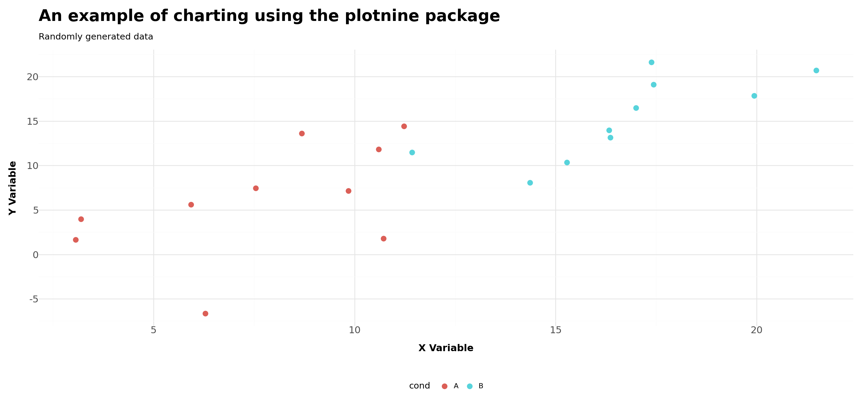
Choice Models and its Applications
Analyzing churn correlation with customer characteristics
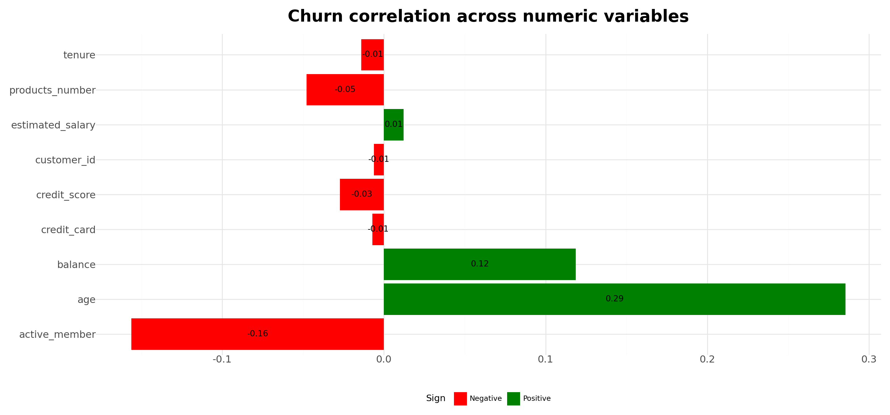
# Select numeric columns and calculate correlation with churn
correlation_df = (
  Data
  .select_dtypes(include='number')
  .corr()
  .iloc[:-1, -1]
  .reset_index()
)

# Rename columns
correlation_df.columns = ['Variable', 'Correlation']

# Add 'Sign' column based on correlation values
correlation_df['Sign'] = correlation_df['Correlation'].apply(lambda x: 'Positive' if x > 0 else 'Negative')

#Chart
Plot = (
  ggplot(correlation_df, aes(x='Variable', y='Correlation', fill='Sign'))+
  geom_col()+
  geom_text(aes(label=correlation_df['Correlation'].round(2)),size=10, color='black',position=position_stack(vjust=0.5))+  # Add annotations
  scale_fill_manual(values=['red','green'])+
  coord_flip()+
  labs(title='Churn correlation across numeric variables')+
  theme_minimal()+
  theme(
    legend_position='bottom',
    axis_title=element_blank(),
    axis_text=element_text(size=12),
    plot_title=element_text(face='bold',size=20),
    figure_size=(15,7)
    )
)

#Display Output
Plot.show()Limitations of the LPM
- Even though we can achieve consistent estimators, we’ll have heteroskedasticity in our estimates by construction. To see that, recall that the conditional expectation of Y given X is given by:
\[ \small E(Y|X)=\underbrace{[P(Y=1|X]}_{X\beta\times 1} + \underbrace{[1-P(Y=1|X)]\times 0}_{=0} = X\beta \]
- Given that the variance of a Bernoulli Distribution is given by \(p \times (1-p)\), then:
\[ V(Y|X)=P(Y|X)\times[1-P(Y|X)]=X\beta\times(1-X\beta) \text{, which clearly depends on } X \]
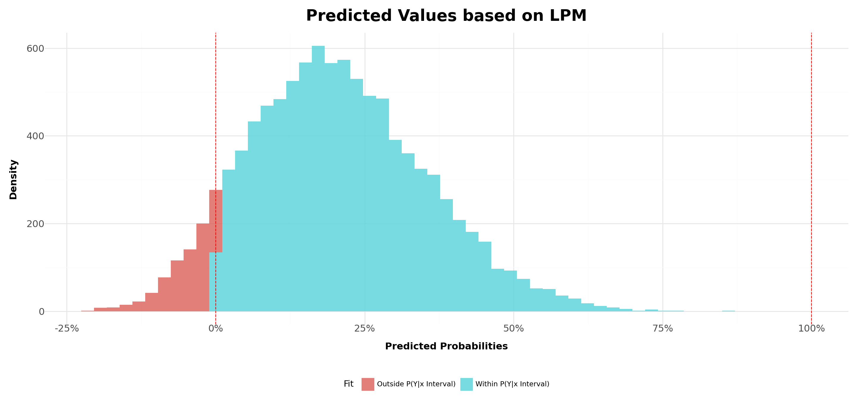
- In most linear probability models, \(R^2\) has no meaningful interpretation:
- Regression line can never fit the data perfectly if the dependent variable is binary and the regressors are continuous
- Since LPM predicts probabilities, the dependent variable is binary (\(0\) or \(1\)), making the interpretation of \(R^2\) problematic. The model often produces predicted values outside the \([0,1]\) range, leading to unreliable goodness-of-fit assessments
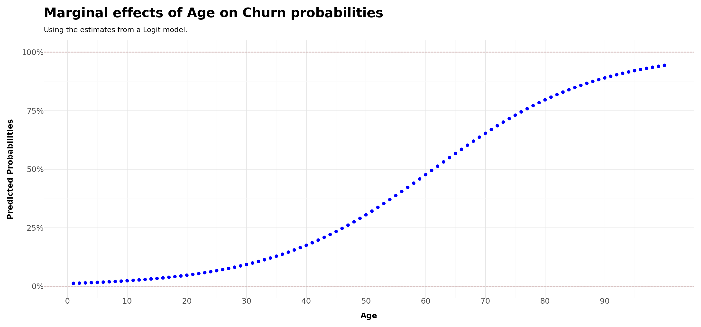
Logit Properties #3: different marginal effects
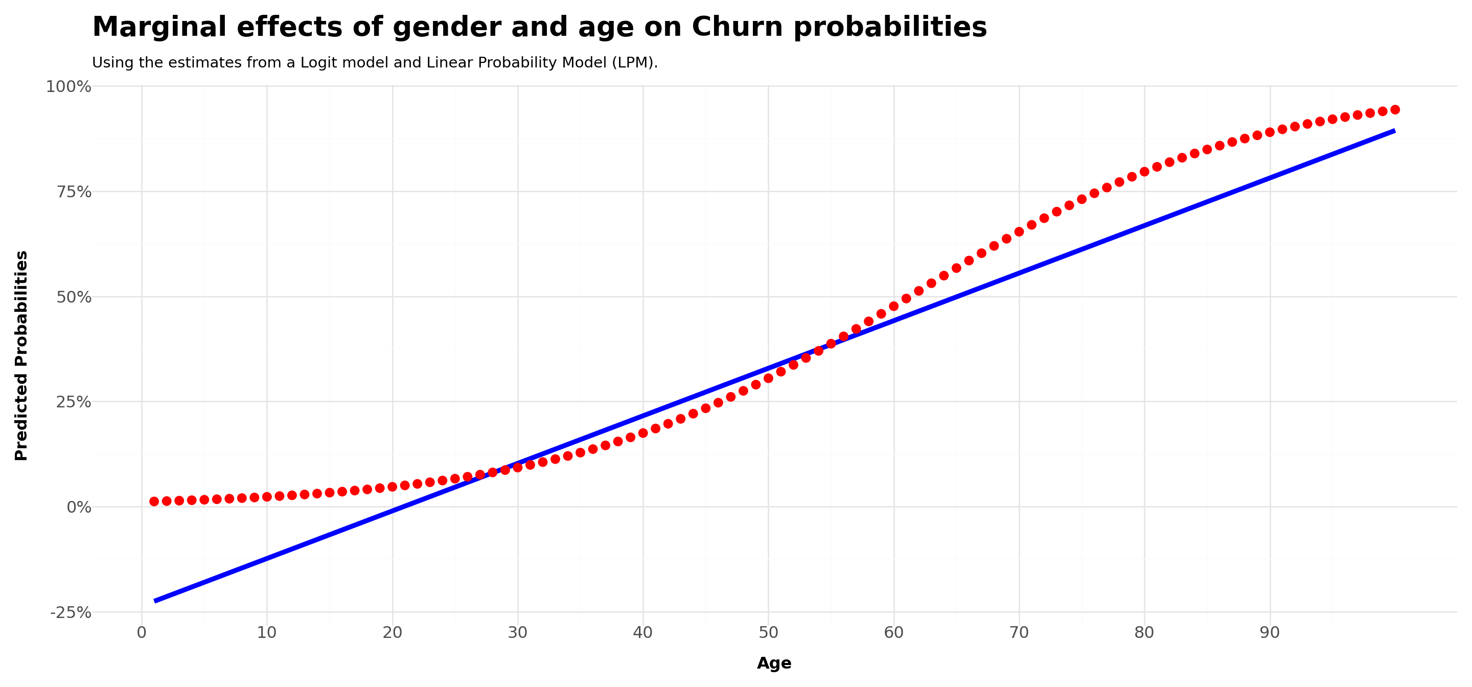
One of the caveats of LPM was that the marginal effect was constant, which does not make a lot of sense from a probabilistic sense
With Logit, the marginal effects are not equal to \(\beta\) anymore. To see that, take the derivative of \(P(Y|X)\) with respect to \(x_1\):
\[ \dfrac{\partial\Lambda(X\beta)}{\partial x_1}=\beta_1 \times\dfrac{\partial\Lambda(X\beta)}{\partial X\beta} \]
As we can see, the effects are not going to be linear anymore!
Put another way, given different levels of X, we may have different marginal effects on the probabilities - in what follows, we’ll analyze the case of
age
# Load data
data = pd.read_csv('Assets/bank-dataset.csv')
data['gender'] = np.where(data['gender'] == 'Male', 1, 0)

# Fit logistic regression model
X = data[['credit_score', 'gender', 'tenure', 'balance', 'products_number', 'credit_card', 'active_member', 'estimated_salary','age']]
X = sm.add_constant(X)  # Add constant term for intercept
y = data['churn']
model = sm.Logit(y, X).fit()

# Set all other variables to the mean
new_data = X.drop(columns=['age']).mean(numeric_only=True).to_frame().transpose()
new_data = pd.DataFrame(np.repeat(new_data.values, 100, axis=0),columns=new_data.columns)
age_df = pd.DataFrame(pd.Series(range(1, 101)), columns=['age'])

# Concatenate with your existing DataFrame
concatenated_df = pd.concat([new_data, age_df], ignore_index=True,axis=1)
concatenated_df.columns=[*new_data.columns,'age']

# Predict on the new data
predicted_df = pd.DataFrame({
    'Age': age_df['age'],
    'Predicted': model.predict(concatenated_df)
    })

# Plot
Plot = (
  ggplot(predicted_df,aes(x='Age',y='Predicted'))+
  geom_point(color='blue',size=2)+
  geom_hline(yintercept=[0,1],linetype='dashed',color='darkred')+
  scale_y_continuous(labels = percent_format())+
  scale_x_continuous(breaks = range(0,100,10))+
  labs(
    title ='Marginal effects of Age on Churn probabilities',
    subtitle = 'Using the estimates from a Logit model.',
    x = 'Age',
    y = 'Predicted Probabilities')+
  theme_minimal()+
  theme(
    legend_position='bottom',
    axis_title=element_text(face='bold',size=12),
    axis_text=element_text(size=12),
    plot_title=element_text(face='bold',size=20),
    figure_size=(15,7)
    )
  )

Plot.show()
Logit Properties #4: different effects by categorical variables
Another interesting use case is to re-do the same analysis before, but now varying also on categorical variables
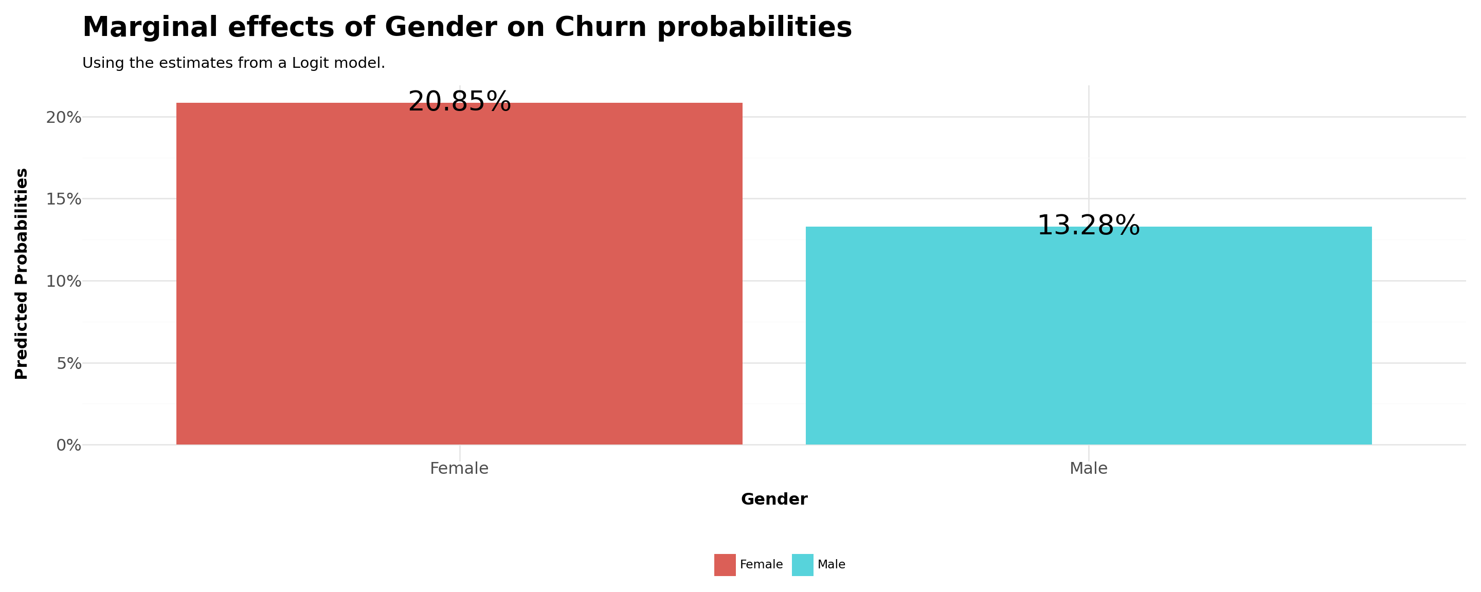
For example, what is the difference in the probability of buying by men and women?
In order to do that, we can set all continous variables to their means and compare the estimated probabilities for
gender=1(male) andgender=0(female)
# Load data
data = pd.read_csv('Assets/bank-dataset.csv')
data['gender'] = np.where(data['gender'] == 'Male', 1, 0)

# Fit logistic regression model
X = data[['credit_score', 'age', 'tenure', 'balance', 'products_number', 'credit_card', 'active_member', 'estimated_salary','gender']]
X = sm.add_constant(X)  # Add constant term for intercept
y = data['churn']
model = sm.Logit(y, X).fit()

# Set all other variables to the mean
new_data = X.drop(columns=['gender']).mean(numeric_only=True).to_frame().transpose()
new_data = pd.DataFrame(np.repeat(new_data.values, 2, axis=0),columns=new_data.columns)
gender_df = pd.DataFrame(pd.Series(range(0, 2)), columns=['gender'])

# Concatenate with your existing DataFrame
concatenated_df = pd.concat([new_data, gender_df], ignore_index=True,axis=1)
concatenated_df.columns=[*new_data.columns,'gender']

# Predict on the new data
predicted_df = pd.DataFrame({
    'Gender': gender_df['gender'],
    'Predicted': model.predict(concatenated_df)
    })

predicted_df['Gender'] = np.where(concatenated_df['gender'] == 1, 'Male', 'Female')

# Plot
Plot = (
  ggplot(predicted_df,aes(x='Gender',y='Predicted',fill='Gender'))+
  geom_col()+
  geom_text(aes(label=predicted_df['Predicted']*100),format_string="{:.2f}%",size=20)+
  scale_y_continuous(labels = percent_format())+
  labs(
    title ='Marginal effects of Gender on Churn probabilities',
    subtitle = 'Using the estimates from a Logit model.',
    x = 'Gender',
    y = 'Predicted Probabilities',
    fill = '')+
  theme_minimal()+
  theme(
    legend_position='bottom',
    axis_title=element_text(face='bold',size=12),
    axis_text=element_text(size=12),
    plot_title=element_text(face='bold',size=20),
    figure_size=(15,6)
    )
  )

Plot.show()
Putting all together
We saw that women tend to churn, approximately, \(8\) percentage points more than men
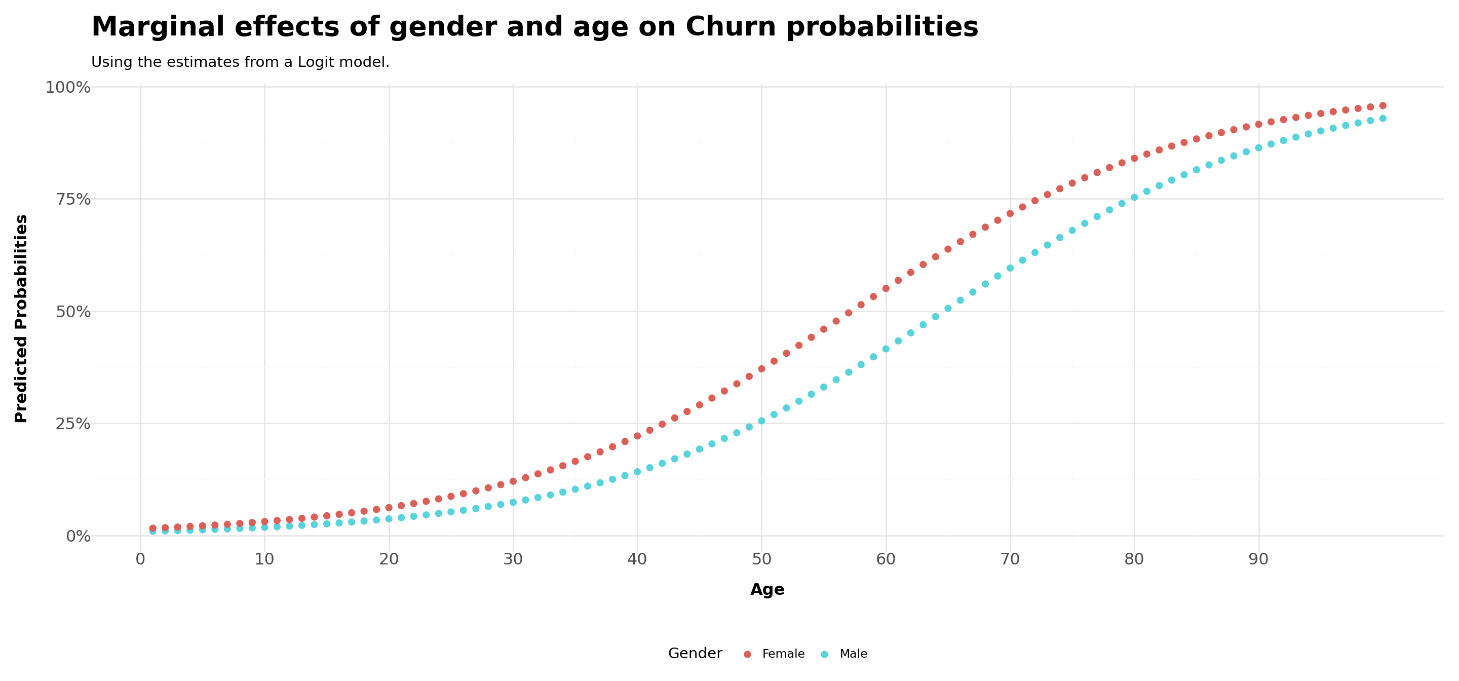
Is this true across all levels of age? As age levels increase, the gap between men and women may become wider due to personal traits. On the other hand, it may be that gender differences are invariant to age
In order to do that, we can do a mix of the two last exercises:
- Set all continuous variables, with the exception of
age, to their means - Compare the estimated probabilities for
gender=1(male) andgender=0(female) - You should have \(200\) rows in your data frame
# Load data
data = pd.read_csv('Assets/bank-dataset.csv')
data['gender'] = np.where(data['gender'] == 'Male', 1, 0)

# Fit logistic regression model
X = data[['credit_score', 'tenure', 'balance', 'products_number', 'credit_card', 'active_member', 'estimated_salary','gender','age']]
X = sm.add_constant(X)  # Add constant term for intercept
y = data['churn']
model = sm.Logit(y, X).fit()

# Set all other variables to the mean
new_data = X.drop(columns=['gender','age']).mean(numeric_only=True).to_frame().transpose()
new_data = pd.DataFrame(np.repeat(new_data.values, 200, axis=0),columns=new_data.columns)
gender_df = pd.DataFrame([*np.repeat(1,100,axis=0),*np.repeat(0,100,axis=0)], columns=['gender'])
age_df = pd.DataFrame(pd.Series(range(1, 101)), columns=['age'])
age_df =pd.concat([age_df,age_df],ignore_index=True,axis=0)

# Concatenate with your existing DataFrame
concatenated_df = pd.concat([gender_df, age_df], ignore_index=True,axis=1)
concatenated_df = pd.concat([new_data,concatenated_df], ignore_index=True,axis=1)
concatenated_df.columns=[*new_data.columns,'gender','age']

# Predict
predicted = model.predict(concatenated_df)
concatenated_df['Predicted'] = predicted
concatenated_df['Gender'] = np.where(concatenated_df['gender'] == 1, 'Male', 'Female')

# Plot
Plot = (
  ggplot(concatenated_df,aes(x='age',y='Predicted',fill='Gender'))+
  geom_point(stroke=0,size=3)+
  scale_y_continuous(labels = percent_format())+
  scale_x_continuous(breaks = range(0,100,10))+
  labs(
    title ='Marginal effects of gender and age on Churn probabilities',
    subtitle = 'Using the estimates from a Logit model.',
    x = 'Age',
    y = 'Predicted Probabilities',
    fill = 'Gender')+
  theme_minimal()+
  theme(
    legend_position='bottom',
    axis_title=element_text(face='bold',size=12),
    axis_text=element_text(size=12),
    plot_title=element_text(face='bold',size=20),
    figure_size=(15,7)
    )
  )

Plot.show()Comparing across LPM and Logit estimations - age
# Read the CSV file into a pandas DataFrame
Data = pd.read_csv('Assets/bank-dataset.csv')

# Convert 'gender' into dummy variables
Data = pd.get_dummies(Data, columns=['gender'], drop_first=True)

# Define independent and dependent variables
X = Data[['credit_score', 'gender_Male', 'tenure', 'balance', 'products_number', 'credit_card', 'active_member', 'estimated_salary','age']]
y = Data['churn']

# Add a constant to the independent variables matrix for the intercept
X = sm.add_constant(X)

# Fit the linear regression model and the logit model
lm_model = sm.OLS(y, X.astype(float)).fit()
logit_model = sm.Logit(y, X.astype(float)).fit()

# Set all other variables to the mean
new_data = X.drop(columns=['age']).mean(numeric_only=True).to_frame().transpose()
new_data = pd.DataFrame(np.repeat(new_data.values, 100, axis=0),columns=new_data.columns)
age_df = pd.DataFrame(pd.Series(range(1, 101)), columns=['age'])

# Concatenate with your existing DataFrame
concatenated_df = pd.concat([new_data,age_df], ignore_index=True,axis=1)
concatenated_df.columns=[*new_data.columns,'age']

# Predict
lm_predicted = lm_model.predict(concatenated_df)
logit_predicted = logit_model.predict(concatenated_df)

predicted_df = pd.DataFrame({
  'LPM': lm_predicted,
  'Logit': logit_predicted,
  'Age': age_df['age']
})


# Plot
Plot = (
  ggplot(predicted_df,aes(x='Age'))+
  geom_line(aes(y='LPM'),color='blue',size=2)+
  geom_point(aes(y='Logit'),color='red',stroke=0,size=4)+
  scale_y_continuous(labels = percent_format())+
  scale_x_continuous(breaks = range(0,100,10))+
  labs(
    title ='Marginal effects of gender and age on Churn probabilities',
    subtitle = 'Using the estimates from a Logit model and Linear Probability Model (LPM).',
    x = 'Age',
    y = 'Predicted Probabilities',
    fill = 'Gender')+
  theme_minimal()+
  theme(
    legend_position='bottom',
    axis_title=element_text(face='bold',size=12),
    axis_text=element_text(size=12),
    plot_title=element_text(face='bold',size=20),
    figure_size=(15,7)
    )
  )

Plot.show()References
![]()
Chapman, Chris, and Elea Mcdonnell Feit. 2015. R for Marketing Research and Analytics. Cham: Springer International Publishing.
Greene, William H. 2011. Econometric Analysis. 7th ed. Upper Saddle River, NJ: Pearson.
Hayashi, Fumio. 2000. Econometrics. Princeton, NJ: Princeton University Press.
Train, Kenneth E. 2009. Discrete Choice Methods with Simulation. 2nd ed. Cambridge, England: Cambridge University Press.