Debt and Taxes

Lucas S. Macoris

Outline

• This lecture is mainly based the following textbooks:

  1. (Berk and DeMarzo 2023)
  2. (Brealey, Myers, and Allen 2020)

• Study review and practice: I strongly recommend using Prof. Henrique Castro (FGV-EAESP) materials. Below you can find the links to the corresponding exercises related to this lecture:

  1. Multiple Choice Exercises - click here

\(\rightarrow\) For coding replications, whenever applicable, please follow this page or hover on the specific slides with coding chunks.

A recap from Modigliani and Miller

• In our previous lecture, we saw the how the Modigliani and Miller propositions played a key role in explaining capital structure decisions:

  1. In perfect capital markets, the total value of a firm’s securities is equal to the market value of the total cash flows generated and is not affected by its choice of capital structure

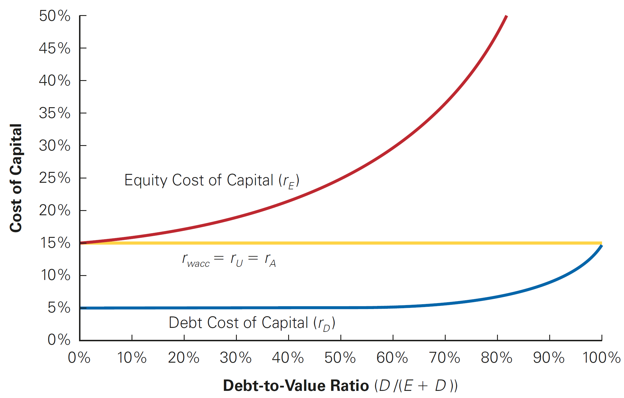
  2. Moreover, the cost of capital of levered equity increases with the firm’s market value debt equity ratio:

\[ \small r_E=r_U+\dfrac{D}{E}(r_U-r_D) \]

\(\rightarrow\) As a consequence, the weighted average cost of capital, WACC, should not be affected by the mix of debt and equity!

WACC dynamics (Perfect Capital Markets)

Why should I bother about Modigliani and Miller?

• You may well think…but we are not in a perfect capital market, so why should I bother? That goes hand in hand with the Modigliani and Miller findings:

  1. If capital markets were perfect (as in the Modigliani and Miller world), then the value of a firm should not be affected by any financial transaction…
  2. … this implies that if there is a financial transaction that appears to be profitable, it must be that it is exploiting some type of market imperfection!

• Knowing how these imperfections affect the firm value is important for business and policy considerations

  1. For example, what happens if you remove the tax-shield from debt interest payments? What if the government decides to tax dividends differently?
  2. These (and other) actions may create/remove market imperfections that will tweak the real-practice results away/closer to the Modigliani-Miller findings!

Reconciling Modigliani and Miller with Debt

Question: if capital structure does not matter, why is debt so abundant?

• The statement that capital structure decisions are irrelevant for the value of a firm are difficult to reconcile with the observation that firms invest significant resources, both in terms of managerial time and effort and investment banking fees, in managing their capital structures

• In many instances, the choice of leverage is of critical importance to a firm’s value and future success:

  1. Firms issue large amounts of debt to pay dividends
  2. Large funds buy companies issuing substantial amounts of debt through leveraged buyouts

\(\rightarrow\) Therefore, if capital structure does matter, then it must stem from a market imperfection!

• In this lecture, we focus on one such imperfection — taxes. As we’ll see, when imperfections from taxes are present, managers can increase the value of a firm through leverage!

The Interest Tax Deduction

• In most cases, firms pay taxes on their profits only after interest payments are deducted
  1. Interest expense reduces the amount of corporate taxes
  2. As a consequence, this creates an incentive to use debt

	With Leverage	Without Leverage
EBIT	$2,800	$2,800
Interest Expenses	-$400	$0
Income before tax	$2,400	$2,800
Taxes (35%)	-$840	-$980
Net income	$1,560	$1,820

• Investors receive \(\small \$1560 + \$400\) (with leverage) versus \(\small \$1820 + 0\) (without leverage). Therefore, in the presence of taxes, leverage increases firm value (equity value + debt value) because the total cash flow received by investors increases!

The Interest Tax Deduction, continued

• We saw that firms can increase value in the presence of taxes through levering up. By how much the firm value increases? You can see that the value of the

\[ \small \underbrace{980}_{\text{Int. Expenses w/o Leverage}} - \underbrace{840}_{\text{Int. Expenses w/ Leverage}} = \underbrace{140}_{\text{Interest Tax-Shield}} \]

• The Interest Tax-Shield is the reduction in taxes achieved due to the higher leverage. Assuming a tax-rate of \(\small 35\%\), we can calculate it as:

\[ \small \text{Tax-Shield}= \tau \times \text{Interest Payments} \rightarrow 35\% \times 400 = 140 \]

• In words, because interest expenses reduce the amount of taxable income, the firm pay less taxes!

Valuing the Interest Tax Shield

• When a firm uses debt, the interest tax shield provides a corporate tax benefit each and every year when interest payments are computed:

  1. It is if the firm was receiving an extra cash flow each year, and this will be used to pay down investors (debtholders + shareholders)

  2. This benefit is then computed as the present value of the stream of future interest tax shields the firm will receive

• As a consequence, the value of the firm, when calculated on the basis of the discounted future cash-flows, will increase due to leverage! Formally, we can reframe our Modigliani-Miller Proposition I in the presence of with taxes: the total value of the levered firm exceeds the value of the firm without leverage due to the present value of the tax savings from debt:

\[ \small \underbrace{V^L}_{\text{Value of Levered Firm}} = \underbrace{V^U}_{\text{Value of Unlevered Firm (all-equity)}} + \underbrace{PV(ITS)}_{\text{Value of Tax-Shields}} \]

Levered and Unlevered Value

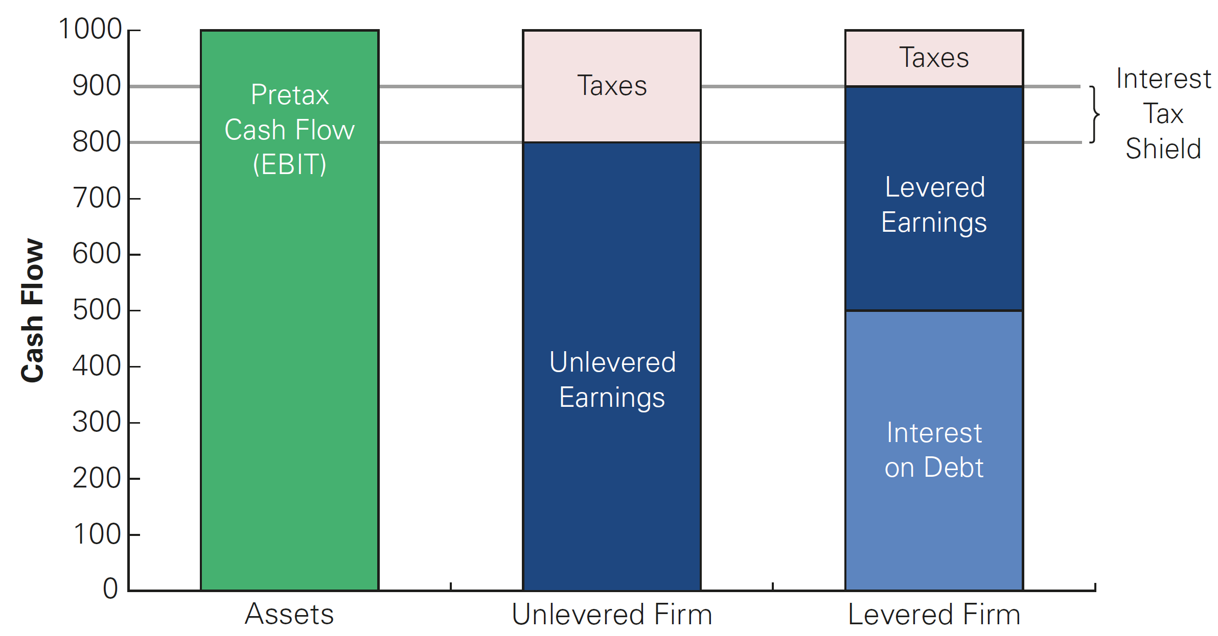
\(\rightarrow\) By increasing the cash flows paid to debt holders through interest payments, a firm reduces the amount paid in taxes!

Valuing the Interest Tax Shield, practice

Suppose ALCO plans to pay 60 million in interest each year for the next eight years, and then repay the principal of 1 billion in year 8. These payments are risk free, and ALCO’s marginal tax rate will remain 39% throughout this period. If the risk-free interest rate is 6%, by how much does the interest tax shield increase the value of ALCO?

\(\rightarrow\) Solution: The annual interest tax shield that is accrued to the firm in from years 1 to 8 is:

\[ \small 1\text{ billion}\times 6\% \times 39\% = 23.4\text{ million} \]

• Therefore, we can calculate the present value of the tax-shields as:

\[ \small PV(ITS) = \frac{23,4}{(1+6\%)^1} + \frac{23,4}{(1+6\%)^2}+. . . + \frac{23,4}{(1+6\%)^8} = 145.31 \text{ million} \]

Valuing the Interest Tax Shield in practice

• When analyzing levered firms, one may think about several debt dynamics that can occurs. Typically, the level of future interest payments is uncertain due to factors such as:

  1. Changes in the marginal tax rate;
  2. Amount of debt outstanding;
  3. Interest rate on the actual debt;
  4. Firm’s risk, among others

• Question: how can we value the interest tax-shield when taking these nuances in consideration? For simplicity, we’ll start by considering the special case in which the above variables are kept constant. This is reasonable because:

  1. Many corporations have policies for fixed amounts of debt
  2. As old bonds and loans mature, new borrowing takes place
  3. Finally, debt can be assumed as permanent, because it is fixed through time

Case I: Valuing the Interest Tax Shield - Permanent Debt

• Suppose a firm borrows a given level of debt \(D\) and keeps the it permanently on its balance-sheets. If the firm’s marginal tax rate is \(\tau_c\), and if the debt is riskless with a risk-free interest rate \(r_f\), then the interest tax shield each year is \(\tau_c \times r_f \times D\), and the tax shield can be valued as a perpetuity:

\[ \small PV(ITS) = \frac{\tau_c \times \text{Int. Expenses}}{r_f} = \frac{\tau_c \times (r_f \times D)}{r_f} = \tau_c \times D \]

• For example, given a \(\small 21\%\) corporate tax rate, this equation implies that for every \(\small \$1\) in new permanent debt that the firm issues, the value of the firm increases by \(\small \$0.21\)!

Valuing the Interest Tax Shield - Dynamics

• You may wonder from where the increased value of the levered firm (\(\small V^L > V^U\)) came from

• It is easy to see that when a firm uses debt financing, the cost of the interest it must pay is offset to some extent by the tax savings from the interest tax shield. Assuming a marginal tax-rate of \(\small \tau_c = 21\%\) and a permanent level of debt \(\small D = 100,000\), at \(\small10\%\) percent interest per year:

Interest expense	$10,000
Tax savings	- $2,100
After-tax cost of debt	$7,900

• Therefore, the effective (or after-tax cost of debt) is:

\[ \small \underbrace{r_d}_{\text{Cost of Debt}} \times \underbrace{(1-\tau_c)}_{\text{Tax-Shield Factor}}\rightarrow 10\%\times(1-21\%)=7.9\% \]

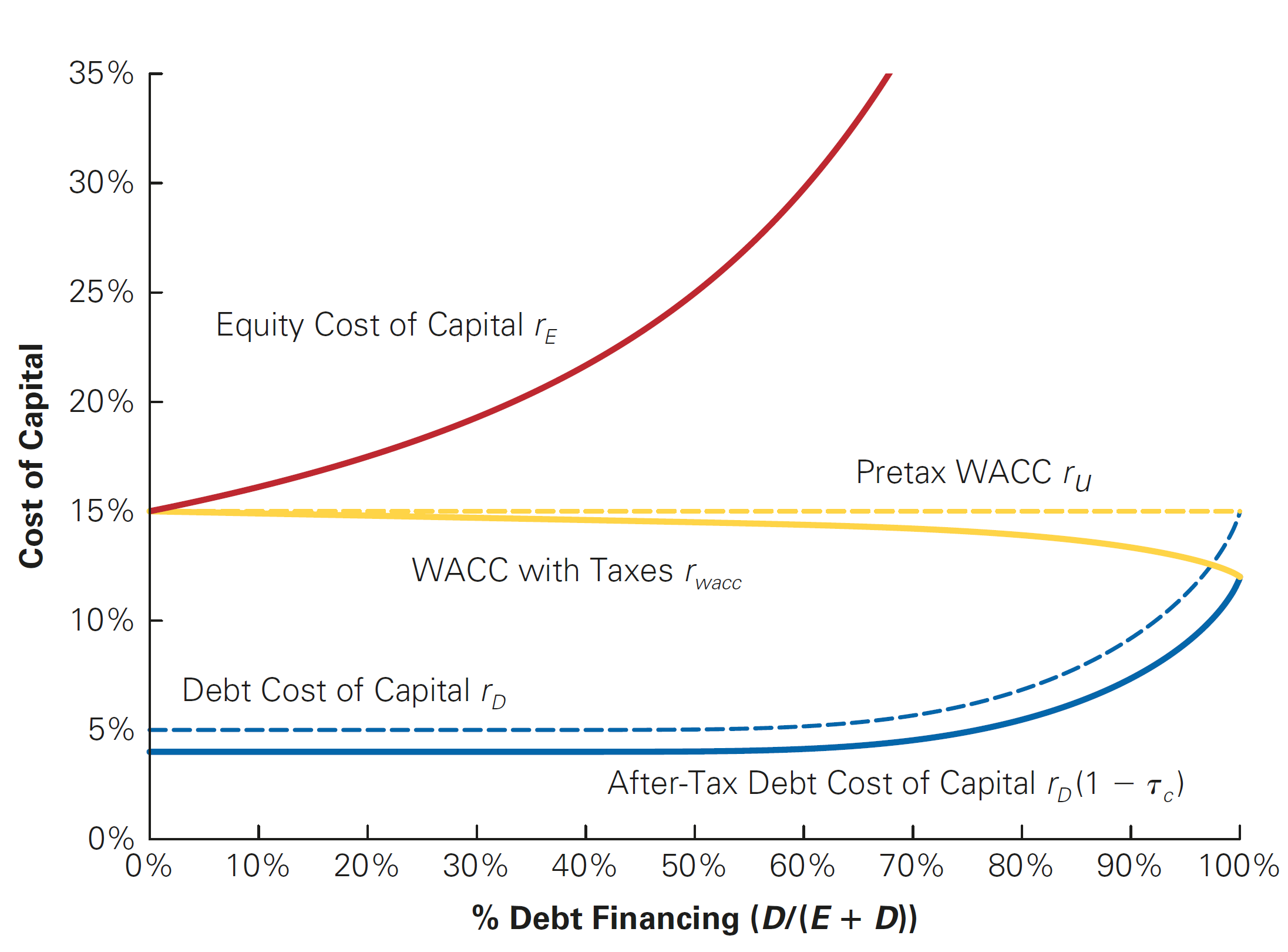
Valuing the Interest Tax Shield - Dynamics (continued)

• Therefore, we can write the After-tax WACC:

\[\small r_{WACC} = \frac{E}{E+D} \times r_e + \frac{D}{E+D} \times r_d \times (1-\tau_c)\]

• More specifically, you can see this in terms of:

\[ \small r_{WACC} = \underbrace{\frac{E}{E+D} \times r_e + \frac{D}{E+D} \times r_d}_{\text{pre-tax WACC}} \underbrace{-\frac{D}{E+D} \times r_d \times \tau_c}_{\text{Reduction due to Interest Tax-Shield}} \]

Valuing the Interest Tax Shield - Dynamics (continued)

Case II: assuming a Target Debt-Equity Ratio

• So far, the value of the tax shield was found assuming a constant level of debt
  1. Instead of assuming a permanent, or fixed value of debt, we can also assume that a firm maintains a constant debt-equity ratio
  2. In other words, although the absolute debt levels change with the size of the firm, the proportions of debt and equity are constant!
• When a firm adjusts its leverage to maintain a target debt-equity ratio, we can compute its value with leverage, \(\small V^L\), by discounting its free cash flow using the after-tax WACC. The value of the interest tax shield can be found by comparing:
  1. The value of the levered firm, \(\small V^L\)
  2. And the value of the unlevered firm, \(\small V^U\)

\[ \small \underbrace{V^L}_{\text{Value of Levered Firm}} = \underbrace{V^U}_{\text{Value of Unlevered Firm (all-equity)}} + \underbrace{PV(ITS)}_{\text{Value of Tax-Shields}} \]

Case II: assuming a Target Debt-Equity Ratio (practice)

Harris Solutions expects to have free cash flow in the coming year of \(\small \$1.75\) million, and its free cash flow is expected to grow at a rate of \(\small 3.5\%\) per year thereafter. Harris Solutions has an equity cost of capital of \(\small 12\%\) and a debt cost of capital of \(\small7\%\), and it pays a corporate tax rate of \(\small 40\%\). If Harris Solutions maintains a debt-equity ratio of \(\small2.5\), what is the value of its interest tax shield?

\(\rightarrow\) Solution: First, compute pre-tax WACC and \(\small V^U\):

\[ \small \text{WACC}_{\text{Pre-Tax}}=\small \frac{E}{E+D} \times r_e + \frac{D}{E+D} \times r_d = \frac{1}{1+2.5} \times 12\% + \frac{2.5}{1+2.5} \times 7\% = 8.43\% \]

• Therefore, the unlevered value, or \(\small V^U\), is:

\[ \small V^U = \frac{1.75}{8.43\% - 3.5\%} = 35.50 \text{ million} \]

Case II: assuming a Target Debt-Equity Ratio (practice)

• We know the value of the unlevered firm. Lnowing that the firm maintains a constant debt-to-equity ratio, the effective cost of debt will be lower due to the tax-shield. We know that the value of the levered firm, \(V^L\), can be found using the after-tax WACC:

\[ \small \text{WACC}_{\text{After-Tax}}=\frac{1}{1+2.5} \times 12\% + \frac{2.5}{1+2.5} \times 7\% \times (1-40\%) = 6.43\% \]

\[ \small V^L = \frac{1.75}{6.43\% - 3.5\%} = 59.73 \text{ million} \]

• As a consequence, the value of the interest tax shield must be:

\[ \small V^L - V^U = 59.73 - 35.50 = 24.23 \text{ million} \]

Recapitalization strategies

• When a firm makes a significant change to its capital structure, the transaction is called a recapitalization (or simply a “recap”)

• For example, in a leveraged recapitalization, a firm issues a large amount of debt and uses the proceeds to pay a special dividend or to repurchase shares

  1. In general, these transactions can reduce firm’s tax payments
  2. But do these transactions ultimately benefit shareholders?

• As we’ll see in the next example, the answer is yes: when we alter the amount of taxes due, the current shareholders of the firm benefit from this change!

Recapitalization strategies - Example

Assume that Midco Industries wants to boost its stock price. The company currently has \(\small 20\) million shares outstanding with a market price of \(\small \$15\) per share and no debt. Midco has had consistently stable earnings and pays a \(\small 21\%\) tax rate. Management plans to borrow \(\small \$100\) million on a permanent basis, and they will use the borrowed funds to repurchase outstanding shares.

• Their expectation is that the tax savings from this transaction will boost Midco’s stock price and benefit shareholders

• Question: is this this expectation realistic?

Recapitalization strategies - Example (continued)

• First, we can calculate the value of Midco Industries without leverage:

\[ \small V^U = 20,000,000 \times 15 = 300 \text{ million} \]

• We know that the present value of the tax-shiedls (after recapitalization) is:

\[ \small \tau_c \times D = 21\% \times 100 \text{ million} = 21 \text{ million} \]

• Therefore, the total value of the levered firm, \(\small V^L\) is:

\[ \small V^L=V^U+PV(ITS)\rightarrow 300+21= 321 \text{ million} \]

Recapitalization strategies - Example (continued)

• Because the value of the debt is \(\small \$100\) million, the value of the equity is:

\[ \small 321 - 100 = 221 \text{ million} \]

• Although the value of the shares outstanding drops from to \(\small \$300\) to \(\small\$ 221\) million, shareholders will also receive \(\small \$100\) million that Midco Industries will pay out through the share repurchases

  1. In total, they will receive the full \(\small \$321\) million, a gain of \(\small \$21\) million over the value of their shares without leverage!

  2. That is, the firm has the incentive to make such recapitalization

Recapitalization strategies - Example (continued)

• Assume Midco Industries repurchases its shares at the current price of \(\small \$15\) per share. The firm will repurchase \(\small 100/15\approx 6.67\) million shares. Therefore, the remaining number of shares is:

\[ \small 20- 6.67= 13.33 \text{ million shares outstanding} \]

• The total value of equity under leverage is \(\small \$221\) million. Therefore, the new share price is:

\[ \small \frac{221}{13.33} = 16.575 \]

• All in all, the total gain to shareholders 21 million, which is exactly the interest tax-shield:

\[ \small (\underbrace{16.575}_{\text{New Price}} - \underbrace{15}_{\text{Prev. Price}}) = \underbrace{1.575}_{\text{Capital Gain}} \times \underbrace{13.33}_{\text{Million Shares}} = 21 \text{ million} \]

Recapitalization strategies - Example (continued)

• In the previous case, the shareholders who remain after the recap receive the benefit of the tax-shield

• However, you may have noticed something odd in the previous calculations…

  1. We assumed that Midco Industries was able to repurchase the shares at the initial price of \(\small \$15\) per share, and then demonstrated that the shares would be worth $16.575 after the transaction

  2. But if the shares are worth \(\small \$16.575\) after the repurchase, why would shareholders tender their shares to Midco at \(\small \$15\) per share?

Recapitalization strategies - Example (continued)

1. In theory, this represents an Arbitrage Opportunity: if investors could buy shares for \(\small \$15\) immediately before the repurchase and sell these shares immediately after at a higher price, this would represent a gain without any risks!

2. In practice, the value of the Midco Industries equity will rise immediately, from \(\small \$300\) million to \(\small \$321\) million, right after the repurchase announcement. In other words, the stock price will rise from \(\small \$15 \rightarrow \$16.05\) immediately!

• With \(\small 20\) million shares outstanding, the share price will rise to: \(\small \$321/20=\$16.05\)

• In other words, Midco Industries must offer at least this price to repurchase the shares, leading to a profit of \(\small \$16.05-\$15=\$1.05\) to shareholders who sell at this price

• Note that all shareholders benefit from this policy: both shareholders who tender their shares and the shareholders who hold their shares both are better-off!

Recapitalization strategies - Example (continued)

1. With a repurchase price of \(\small \$16.05\), both shareholders who tender their shares and the ones who hold their shares both gain \(\small \$16.05 − \$15 = \$1.05\) per share as a result of the transaction

2. The benefit of the interest tax shield goes to all \(\small 20\) million shares outstanding for a total benefit of:

\[ \small \underbrace{1.05}_{\text{Gain per share}}\times \underbrace{20}_{\text{Shares Outstanding}} = \underbrace{21 \text{ million}}_{\text{Interest Tax-Shield}} \]

\(\rightarrow\) When securities are fairly priced, the original shareholders of a firm capture the full benefit of the interest tax shield from an increase in leverage!

\(\rightarrow\) See (Berk and DeMarzo 2023), page 566, for a more comprehensible simulation for different values of tender prices

Practical Exercise

Assume that a firm maintains a debt-equity ratio of \(\small0.85\), and has an equity cost of capital of \(\small12\%\), and a debt cost of capital of \(\small7\%\). The applicable corporate tax rate is \(\small25\%\), and its market capitalization is \(\small\$220\) million. If the firms’ free cash flow is expected to be \(\small\$10\) million in one year, what constant expected future growth rate is consistent with the firm’s current market value?

\(\rightarrow\) Solution: first, we calculate the WACC as:

\[ \small \text{WACC}= \dfrac{1}{1+0.85}\times 12\% + \dfrac{0.85}{1+0.85}\times 7\% \times (1-25\%)=8.90\% \]

Note that \(\small V^L=E+D\). If the market capitalization is \(\small 220\), then \(\small D = E\times 0.85=187\). Therefore, the firm value can be estimated in terms of a growing perpetuity:

\[ \small V^L=\dfrac{FC}{r-g}= (220+187)=\dfrac{10}{8.90\%-g}\rightarrow g \approx 6.44\% \]

Practical Exercise

Based on the previous exercise, estimate the value of firm’s interest tax shield.

\(\rightarrow\) Solution: first, we calculate the pre-tax WACC (or \(\small r_U\)) as:

\[ \small \text{pre-tax WACC}= \dfrac{1}{1+0.85}\times 12\% + \dfrac{0.85}{1+0.85}\times 7\%=9.70\% \]

Remember that you can find the value of unlevered equity (\(\small V^U\)) by discounting using the unlevered cost of capital (or pre-tax WACC):

\[ \small V^U=\dfrac{10}{9,7\%-6.44\%}= 307 \] Therefore, the present value of the interest tax shield is simply the difference between the levered and unlevered equity:

\[ \small PV(ITS)=V^L-V^U\rightarrow 407-307=100 \]

Accounting for Personal Taxes

• So far, we have looked to the benefits of leverage in the presence of corporate taxes. Although it is correct to say that the firm has a higher cash flow due to tax-shield savings, it is not straightforward to say that shareholders are fully benefiting from such increase

• What happens to our conclusions on debt benefits when we account for the effect of personal taxes?

  1. The rate that corporations paid as tax is usually different than that investors pay
  2. Additionally, the cash flows to investors are typically taxed twice. Once at the corporate level and then investors are taxed again when they receive their interest or divided payment

\(\rightarrow\) Since personal taxes have the potential to offset some of the corporate tax benefits of leverage, in order to determine the true tax benefit of leverage, we need to evaluate the combined effect of both corporate and personal taxes!

Accounting for Personal Taxes, continued

• In the United States and many other countries, interest income has historically been taxed more heavily than capital gains from equity¹

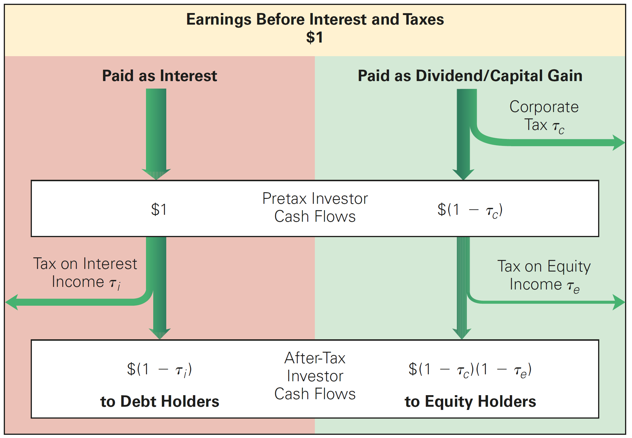
• To determine the true tax benefit of leverage, we need to evaluate the combined effect of both corporate and personal taxes. In order to see that, consider a firm with \(\small\$1\) of earnings before interest and taxes (EBIT). The firm has two options:

  1. The firm can either pay this \(\small\$1\) to debt holders as interest
  2. Alternatively, it can be used pay equity holders directly - either directly, with a dividend, or indirectly, by retaining earnings

• Depending on the type of investor, tax rates are different:

  1. For a debtholder, the amount paid net of taxes is \(\small(1-\tau_i)\)
  2. For an equityholder, not only the firm pays \(\small \tau_c\) on its taxable income, but individuals are taxed by \(\small \tau_e\) at a personal level: \(\small (1-\tau_c)\times(1-\tau_e)\)

1. Note that, in Brazil, dividends are not taxed.

Comparing after-tax cashflows

• We can summarize the previous example using U.S. tax rates as of 2018:

Payment Due	After-Tax Cash Flows	Using Current Tax Rates
To debt holders	\(\small(1 −\tau_i)\)	( 1 − 0.37 ) = 0.63
To equity holders	\(\small(1 − \tau_c)\times(1-\tau_e)\)	(1 − 0.21)( 1 − 0.20 ) = 0.632

• Based on this, we can write:

\[ \small (1-\tau^*) \times (1-\tau_i) = (1-\tau_c)\times(1-\tau_e) \]

• We can interpret \(\small \tau^*\) as the effective tax advantage of debt: if the corporation paid \(\small (1-\tau^*)\) in interest, debt holders would receive the same amount after taxes as equity holders would receive if the firm paid \(\small \$1\) in profits to equity holders

Accounting for Personal Taxes, continued

Tax advantages of debt

• Using this structure, we can calculate the Effective Advantage of Debt as follows:

\[ \small \tau^* = 1-\frac{(1-\tau_c)\times(1-\tau_e)}{(1-\tau_i)} \]

• Finally, notice that if interest payments and equity payment tax burdens are equivalent, debt policy is irrelevant:

\[ \small(1-\tau_e) \times (1-\tau_c) = (1-\tau_i) \]

Accounting for Personal Taxes, practice

Assume that the corporate tax rate (\(\small \tau_c\)) is \(\small 34\%\), the personal tax rate on equity (\(\small \tau_e\)) is \(\small 28\%\), and the personal tax rate on debt (\(\small \tau_i\)) is also \(\small 28\%\). What is the tax advantage of debt for a firm?

\(\rightarrow\) Solution: using the formula, we have that:

\[ \small \tau^* = 1-\frac{(1-\tau_c)\times(1-\tau_e)}{(1-\tau_i)}\rightarrow 1-\dfrac{(1-34\%)\times(1-28\%)}{(1-28\%)}=34\% \]

• In other words, the tax advantage of debt is the corporate tax rate if there is no difference between the tax rate on interest payments or equity

• If, for example, equity income is taxed less heavily than interest income, then \(\small \tau^\star\), the tax advantage of debt, will be lower than the corporate tax rate

Accounting for Personal Taxes, practice

• Consider the stylized Brazilian case and compute the effective tax advantage of debt.

  1. Personal tax rate: \(\small \tau_i = 27.5%\)
  2. Equity income tax rate: \(\small \tau_e= 15\%\)
  3. Corporate tax rate: \(\small \tau_c = 34\%\)

• The tax advantage of debt in a Brazilian setting is:

\[ \small \tau^* = 1-\frac{(1-34\%)\times(1-15\%)}{(1-27.5\%)} = 22.6\% \]

Practical implications Personal Taxes

• There is a rationable to argue that that tax advantages of debt differ across investors:
  1. Tax rates vary for individual investors, and many investors are in lower tax brackets
  2. Holding periods might also have an effect on personal taxes
• Given the wide range of tax preferences and brackets across investors, it is difficult to know the true value of \(\tau^*\) for a firm
  • Using the top personal tax rates likely understates \(\tau^*\)
    
  • Ignoring personal taxes likely overstates \(\tau^*\)

Personal Taxes and Firm Value

• We now can write:

\[V^L = V^U + \tau^* \times D\]

• We still compute the WACC using the corporate tax rate \(\tau_c\).
  • With personal taxes the firm’s equity and debt costs of capital will adjust to compensate investors for their respective tax burdens
  • The net result is that a personal tax disadvantage for debt causes the WACC to decline more slowly with leverage than it otherwise would.

Estimating the Interest Tax Shield with Personal Taxes

MoreLev Inc. currently has a market cap of \(\small\$500\) million with \(\small40\) million shares outstanding. It expects to pay a \(\small 21\%\) corporate tax rate. It estimates that its marginal corporate bondholder pays a \(\small20\%\) tax rate on interest payments, whereas its marginal equity holder pays on average a \(\small10\%\) tax rate on income from dividends and capital gains. MoreLev plans to add permanent debt. Based on this information, estimate the firm’s share price after a \(\small\$220\) million leveraged recap.

\(\rightarrow\) Solution: using the formula for the tax advantage of debt, we have that:

\[ \small \tau^* = 1-\frac{(1-21\%)\times(1-10\%)}{(1-20\%)} = 11.1\% \]

• Therefore, having debt in the firm’s capital structure increases the firm’s value to:

\[ \small \tau^\star\times D \rightarrow 11.1\%\times 220 = 24.4 \text{ million} \]

• Share prices rise by \(\small \$24.4/40\approx\$0.61\), and the new share price is \(\small \$12.5+\$0.61 = \$13.11\)

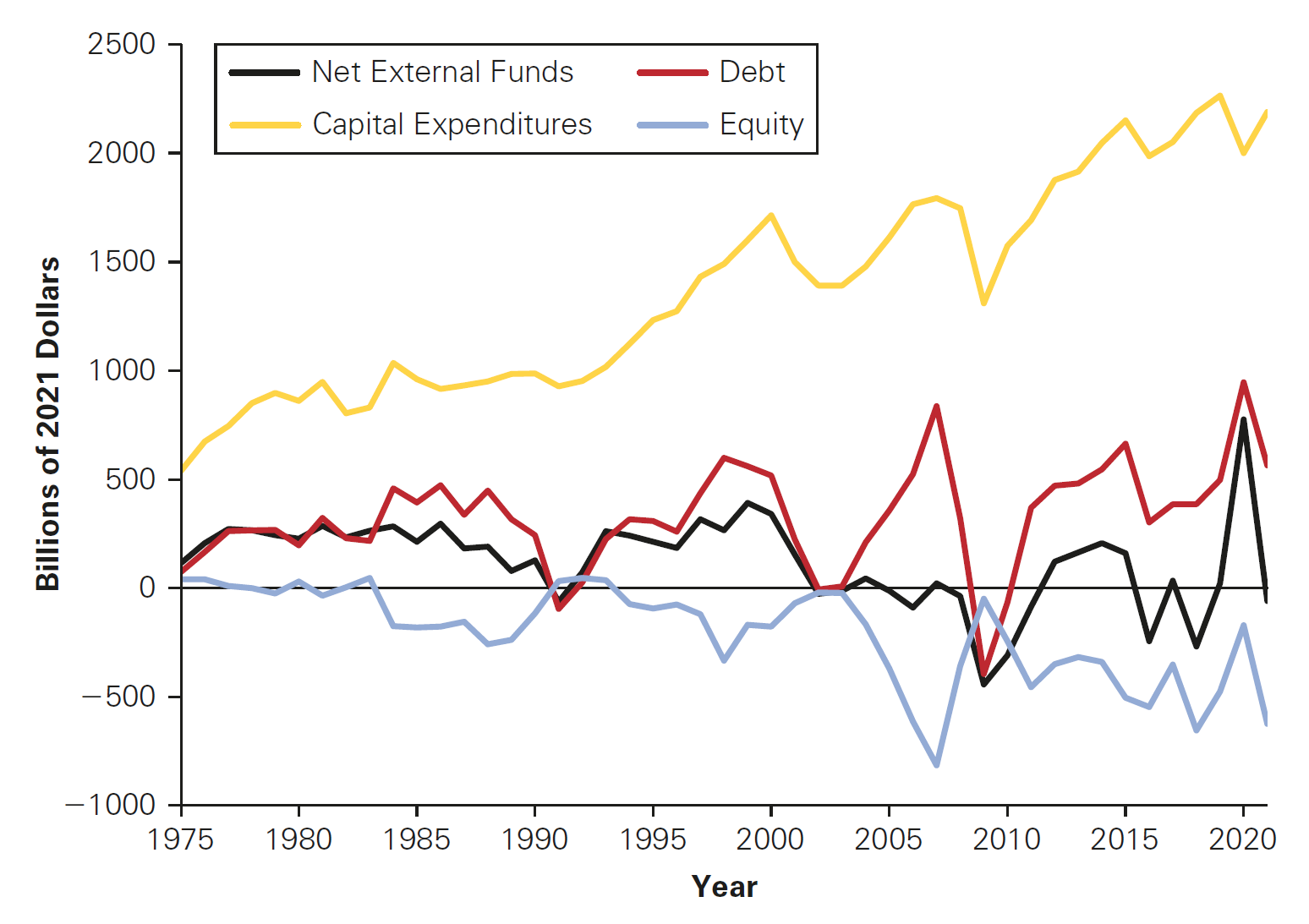
Do firms prefer Debt? Equity and Debt issuances

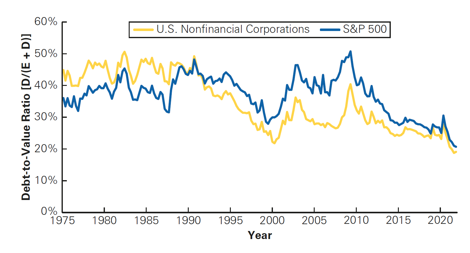
Do firms prefer Debt? Debt-to-Value ratios

Do firms prefer Debt? The Cross-section of Debt Ratios

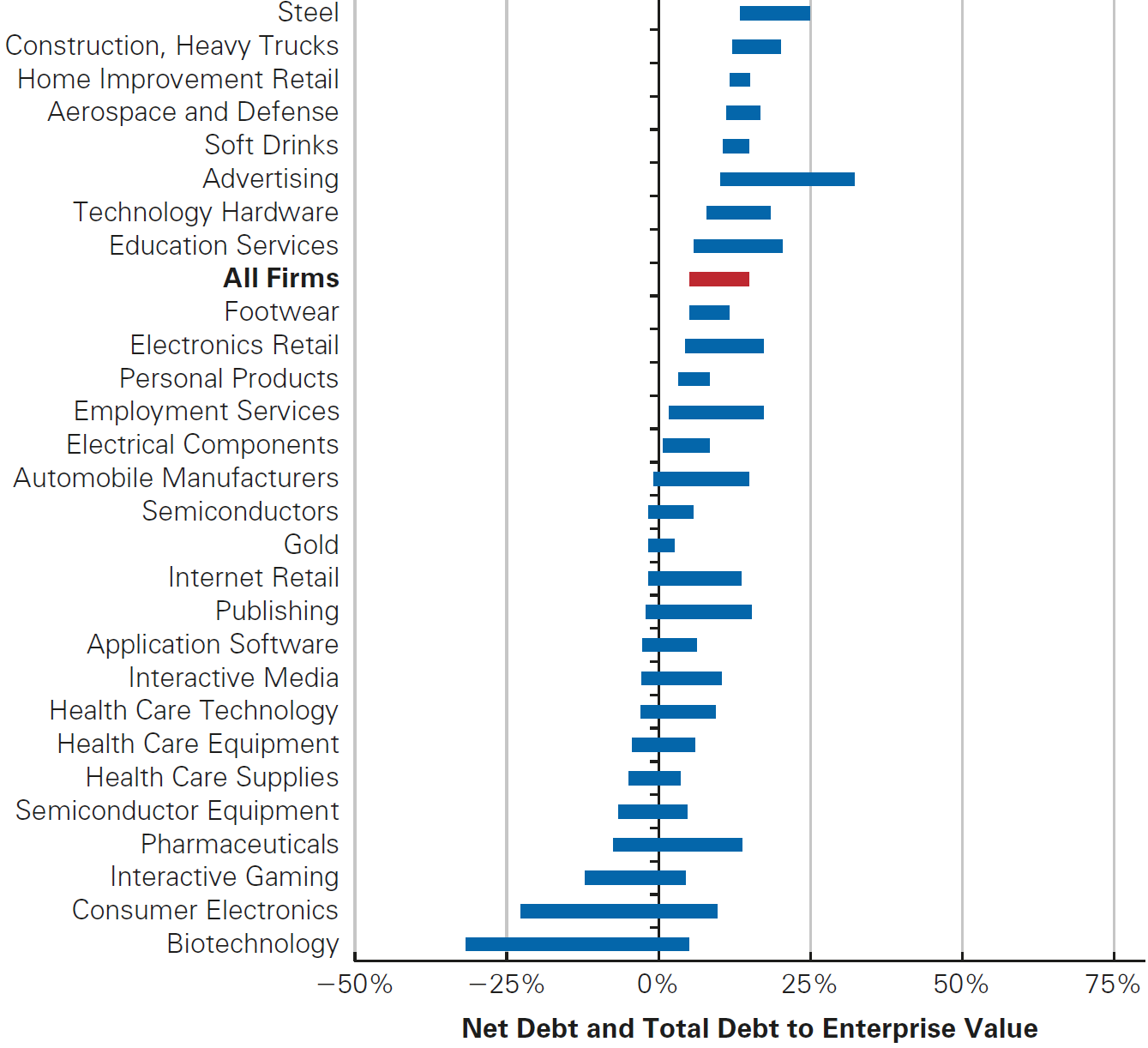
Note: full picture in (Berk and DeMarzo 2023)

Optimal Capital Structure with Taxes

• The evidence from the U.S. market outlined in the previous three slides shows us that:
  1. For the average firm, the result is that debt as a fraction of firm value has varied in a range from 30% to 45%
  2. The use of debt varies greatly by industry
  3. Firms in growth industries like biotechnology or high technology carry very little debt, while airlines, automakers, utilities, and financial firms have high leverage ratios
  4. Finally, many firms hold huge amounts of cash, actually making net debt negative

Question: considering all the tax benefits of debt, why is that firms do not use more debt?

\(\rightarrow\) A potential explanation (among other hypotheses) is that there are limits to the tax benefit of debt that makes firm to optimally set a given debt-to-value ratio

Limits to tax benefits

• When it comes to taxable earnings, there may be limits to how much a firm can deduct interest expenses on its taxable income - in our case, EBIT

  1. To receive the full tax benefits of leverage, a firm need not use 100% debt financing, but the firm does need to have taxable earnings
  2. This constraint may limit the amount of debt needed as a tax shield

• For example, in the United States, there is a limit of \(\small 30\%\) of the EBIT for how much can be deducted in taxable income due to interest payments¹

• Consider a case where EBIT is \(\small \$1,000\) and the corporate tax rate is \(\small 21\%\). In a situation like this, a firm may limit its leverage to achieve the highest interest shield possible from a tax perspective - see Table in the next slide

1. Interest deductions in excess of the 30% limit can be carried forward and used the next time the firm does not exceed the limit. This delay reduces the present value of the tax benefit (and it may ultimately be lost if the firm’s interest coverage remains too low)

Limits to tax benefits - example

	No Leverage	Moderate Leverage	Excess Leverage
EBIT	$1,000	$1,000	$1,000
Interest Expenses	$0	$300	$500
30% Limit	$300	$300	$300
Interest Deduction	$0	$300	$300
Taxable Income	$1,000	$700	$700
Taxes (21%)	$210	$147	$147
Net Income	$790	$553	$353
Tax Shield	$0	$63	$63

\(\rightarrow\) The optimal level of leverage from a tax saving perspective is the level such that interest just equals the income limit

Growth and Debt

• How firms could optimally set their leverage from a tax savings perspective? A way to think about it is to relate to its future EBIT (taxable earnings):

  1. Growing firms often have no taxable earnings and therefore do not use much debt
  2. At the optimal level of leverage, the firm shields all of its taxable income, and it does not have any tax-disadvantaged excess interest
  • However, it is unlikely that a firm can predict its future EBIT (and the optimal level of debt) precisely
  • If there is uncertainty regarding EBIT, then there is a risk that interest will exceed EBIT
  • As a result, the tax savings for high levels of interest falls, possibly reducing the optimal level of the interest payment

\(\rightarrow\) In general, as a firm’s interest expense approaches its expected taxable earnings, the marginal tax advantage of debt declines, limiting the amount of debt the firm should use

Wrapping-up: the Low leverage puzzle

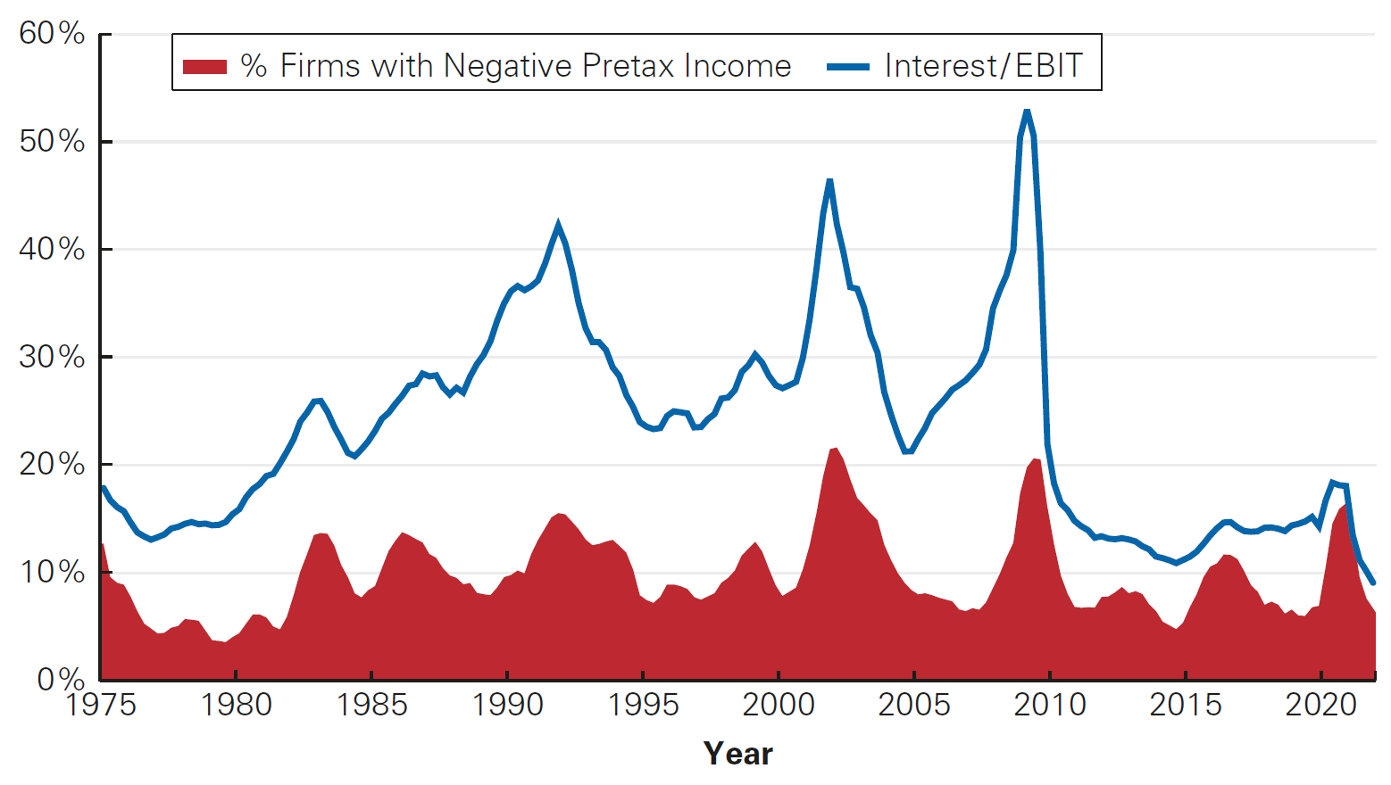
\(\rightarrow\) It seems that firms are under-leveraged consistently. Therefore, there must be more to this capital structure story

Practice

• Take a look at an example of a Debenture Prospectus for Raízen S.A - access here

• Read more about the dispute between BTG Pactual and Americanas S.A on an accelerated repayment agreement close to when news about the firm’s accounting inconsistencies became public - access here

Important

Practice using the following links:

1. Multiple-choice Questions

References

Berk, J., and P. DeMarzo. 2023. Corporate Finance, Global Edition. Global Edition / English Textbooks. Pearson. https://books.google.com.br/books?id=m78oEAAAQBAJ.

Brealey, R. A., S. C. Myers, and F. Allen. 2020. Principles of Corporate Finance. The Irwin/McGraw-Hill Series in Finance, Insurance, and Real Estate. McGraw-Hill Education. https://books.google.com.br/books?id=nsrHuwEACAAJ.