Optimal Portfolio and the CAPM

Lucas S. Macoris

Outline

• This lecture is mainly based the following textbooks:

  1. (Berk and DeMarzo 2023)
  2. (Brealey, Myers, and Allen 2020)

• Study review and practice: I strongly recommend using Prof. Henrique Castro (FGV-EAESP) materials. Below you can find the links to the corresponding exercises related to this lecture:

  1. Multiple Choice Exercises - click here
  2. Numeric Exercises - click here

\(\rightarrow\) For coding replications, whenever applicable, please follow this page or hover on the specific slides with coding chunks

From Assets to Portfolios

The Expected Return of a two-stock portfolio

• Previously, we looked at returns from individual assets, but investors are always looking for ways to invest in multiple assets at the same time. What if you hold a portfolio of \(n\) assets?

• Let’s keep it simple for now. Suppose you have a two-stock portfolio of assets that hipotetically consists of:

  1. Amazon (AMZN) 40% of the portfolio, 10% return and standard deviation (volatility) of 25%
  2. Ferrari (RACE): 60% of the portfolio, 15% return and stardard deviation (volatility) of 30%

• If your portfolio is 40% Amazon and 60% Ferrari, then the return of your portfolio, \(R_p\) is:

\[\small R_p= \sum_{i=1}^{2}\big(x_i\times R_i\big)=(0.4 \times 10\%) +(0.6 \times 15\%) = 13\%\]

\(\rightarrow\) In other words, the return of a portfolio is the weighted average of the individual asset returns!

The Expected Return of a two-stock portfolio, continued

Important

The weights are selected by the investors and may change over time if the prices change (unless the investor actively rebalances it to match the same proportion by buying/selling). Without trading, the weights increase for those stocks whose returns exceed the portfolio’s return.

• To see that, assume that your initial holdings are $100,000:

  1. If Amazon is 40% of the portfolio with a 10% return \(\small \rightarrow 40,000\times (1+10\%)=44,000\)
  2. If Ferrari is 60% of the portfolio with a 15% return \(\small \rightarrow 60,000\times (1+15\%)=69,000\)

• Your holdings are now worth \(\small 44,000 + 69,000= 113,000\), which yields the 13% return, but now the weights from each stock are different:

  1. Amazon holdings are \(\small \frac{44}{113}\approx 38.9\%\) of the portfolio
  2. Ferrari holdings are \(\small \frac{69}{113}\approx 61.1\%\) of the portfolio

Volatility of a two-stock portfolio

• As we now have a portfolio of two different assets, what should be the volatility? Recall that:

  1. Amazon (AMZN)’s standard deviation (volatility) was hipothetically 25%
  2. Ferrari (RACE)’s stardard deviation (volatility) was hipothetically 30%

• As we’ll see in the next slides, to compute the standard deviation of a portfolio, we cannot rely on the weighted average anymore!

• In order to see that, let’s look at the historical prices from both stocks and compare:

  1. The price trend from Amazon
  2. The price trend from Ferrari
  3. The dollar holdings for a portfolio of $100 that holds 40% Amazon and 60% Ferrari

• In what follows, we’ll see how these dynamics shed light on the covariance of the portfolio

Volatility of a two-stock portfolio, historical trends

Volatility of a two-stock portfolio, summary statistics

• If we now look at the annualized statistics, we see that..

1. The weighted average between the individual volatilies is around 25.9%
2. But our portfolio volatility is lower than the individual volatilities. Why? Diversification!

• Intuitively, the returns from both stocks do not move in lockstep: whenever Ferrari prices goes down, Amazon prices move in a different fashion

• In fact, the correlation between the returns of these stocks is around 0.39. In other words, these assets do not move in the same direction all the time!

An interlude: Variance, Covariance, and Correlation

• You can find the proofs for both definitions in the Appendix

Definition

1. The Variance (\(\sigma^2\)) is the squared deviations of the returns from their means: \(\small E[X-E(X)]^2\)
2. Covariance (\(Cov\)) is the expected product of the deviations of two returns from their means: \(\small [X-E(X)][Y-Y(X)]\)

Theorem I: the variance of the sum of two random variables equals the sum of the variances of those random variables, plus two times their covariance:

\[ \sigma^2(A+B) = \sigma^2_A + \sigma^2_B + 2\times Cov(A,B) \]

Theorem II: The variance scales upon multiplication with a constant:

\[ \sigma^2(\beta \times A ) = \beta^2\times \sigma^2_A \]

Volatility of a two-stock portfolio, continued

• Let’s now apply this to understand our portfolio’s volatility using daily data. Define:

  1. \(\sigma^2_1\) = variance of Asset 1 (Amazon).
  2. \(\sigma^2_2\) = variance of Asset 2 (Ferrari)
  3. \(\sigma_{1,2}\) = covariance between both assets
  4. \(w_1\) and \(w_2\) are the weights for both assets

• Using the definitions highlighted before, that the variance of our portfolio returns, \(R_p\), is:

\[ \small \sigma^2(R_p)=\sigma^2(w_1\times R_1+w_2\times R_2)=w_1^2\times \sigma^2_1 + w_2^2 \times \sigma^2_2 + 2\times w_1\times w_2\times \sigma_{1,2} \]

Variance in terms of correlation

• We can further simplify this using the fact that the Covariance is the product of the assets’ standard deviations and their correlation:

\[ \small \sigma^2(R_p)=w_1^2\times \sigma^2_1 + w_2^2 \times \sigma^2_1 + 2\times w_1\times w_2\times \underbrace{Cov(R_1,R_2)}_{\sigma_1 \times \sigma_2 \times Corr_{12}}\\ \small = \underbrace{w_1^2\times \sigma^2_1}_{1} + \underbrace{w_2^2 \times \sigma^2_1}_{2} + \underbrace{2\times w_1\times w_2\times \sigma_1 \times \sigma_2 \times Corr_{12}}_{3} \]

1. The first term relates to the first asset (in our case, Amazon) variance and its proportion in the portfolio
2. The second term relates to the second asset (in our case, Ferrari) variance and its proportion in the portfolio
3. The third term relates to the relationship between both assets

A note on sample analogues

• Recall that we cannot rely on expectations to future outcomes and/or probabilities to calculate the expected returns of the portfolio and its volatility

• Because of that, as we did before, we replace the expectation estimator, \(E(\cdot)\), with our sample analogue, which is the sample average, and it is always backward-looking:

  1. Fix a period for calculation (for example, the latest 30 days)
  2. Calculate the risk and return using sample averages

• To facilitate the notation, we’ll always refer to it using a bar: \(\overline{R}\). For example the covariance between the returns from stocks \(i\) and \(j\) is:

\[Cov(R_i,R_j) = \frac{\sum_{1}^{T}(R_i-\overline{R_i} ) \times (R_j-\overline{R_j})}{T-1}\]

Getting back to our portfolio

• Using our formula for the variance of the portfolio:

\[ \small \sigma^2_p= w_1^2\times \sigma^2_1 + w_2^2 \times \sigma^2_1 + 2\times w_1\times w_2\times \sigma_1 \times \sigma_2 \times Corr_{12}\\ \small \underbrace{\small 0.4^2\times 0.3290^2+0.6^2\times 0.2124^2}_{I} + \underbrace{2\times 0.4\times0.6\times 0.3290\times 0.2124\times 0.3886}_{II} = 0.04659402 \]

• Therefore, \(\sigma_{p}\) is simply \(\small \sqrt{0.04659402}=0.2159\) or 21.59%. You could also calculate the daily portfolio variance and annualize it at the end multiplying it by \(\sqrt{n}\)

Variance of a 2-stock portfolio, continued

• Looking at our formula, we have:

\[ \small \sigma^2_p= w_1^2\times \sigma^2_1 + w_2^2 \times \sigma^2_1 + 2\times w_1\times w_2\times \sigma_1 \times \sigma_2 \times Corr_{12}\\ \small \underbrace{\small 0.4^2\times 0.3290^2+0.6^2\times 0.2124^2}_{I} + \underbrace{2\times 0.4\times0.6\times 0.3290\times 0.2124\times 0.3886}_{II} = 0.04659402 \]

1. The first term (I) captures the individual variances contribution
2. The second term (II) captures the relationship between assets (note that 0.3312 is the correlation between both individual returns)

Wrapping up - 2-stock portfolio volatility

• These assets have roughly similar historical return and volatility, but they ‘move’ very differently:

1. For example, when Amazon performed well, Ferrari did not move in lockstep
2. As a matter of fact, their correlation is about 0.39, meaning that their prices do not trend in the same direction most of the time!

• As you now see, the return of the portfolio is equal to the weighted average of the individual returns…

• …However, the volatility of is much lower than the volatility of the two individual stocks, as the assets are offseting each other and making the return “smoother”!

• How much risk is eliminated when creating a portfolio? It depends on the degree to which the stocks face common risks and their prices move together (in mathematical terms, this will be captured by the correlation parameter, \(\small Corr_{12}\)!

Volatility of a large portfolio

• What if we added a third asset to our portfolio? Let’s say that you’re really into discretionary goods and decide to place a bet on Victoria’s Secret (ticker: VSCO), which had 30% of return in the previous last

• You decided to keep the weight on Amazon and split Ferrari and Victoria’s Secret evenly, with 30% each

• How does that play a role in your portfolio? As before, your portfolio Return is simply a weighted average of the individual returns:

\[ R_{p}=\sum_{i=1}^{3}w_i\times R_i = \underbrace{(0.4 \times 10\%)}_{\text{Amazon}} +\underbrace{(0.3 \times 15\%)}_{\text{Ferrari}}+ \underbrace{(0.3 \times 25\%)}_{\text{VSCO}}\approx 16\% \]

• Let’s see how this strategy performed from 2023 up to now!

Ouch! You’ve seen to be worse off now!

Your VSCO bet did not play well, unfortunately

• Adding VSCO to the portfolio severely hit the overall return, \(\small R_p\)

• VSCO was also very volatile: its standard deviation was twice as high as Amazon. However, the portfolio volatility is substantially lower

• One way to understand this is to look at the correlation matrix between the assets

VSCO is not strongly correlated with the other assets

• Looking at the correlation matrix, we can see that:
  1. \(\small Corr_{\text{AMZN,VSCO}}=0.16\)
  2. \(\small Corr_{\text{RACE,VSCO}}=0.14\)
• As we can see, because the correlation coefficient is very small, the contribution of VSCO to the overall portfolio volatility is limited

The variance of a 3-stock portfolio

• How can we extend your variance calculation for three assets?

• The general formulation of the variance formula shows us that:

\[ \small Var(X)=Var(A+B+C) = E[((A+B+C)-E(A+B+C))]^2 =\\ \small E[(\underbrace{[A-E(A)]}_{\text{First Term}}+[\underbrace{B-E(B)}_{\text{Second Term}}]+[\underbrace{C-E(C)}_{\text{Third Term}}])^2] \\ \]

• This is a quadratic form, and we can decompose it as:

\[ \small (A+B+C)^2= A^2+B^2+C^2 + 2AB + 2AC +2BC \]

The variance of a 3-stock portfolio, continued

• In portfolio terms:

\[ \small \sigma^2_p= \underbrace{w_1^2\times \sigma^2_1}_{I} + \underbrace{w_2^2 \times \sigma^2_1}_{II} \small + \underbrace{w_3^2 \times \sigma^3_1}_{III} \\ \small + \underbrace{2\times w_1\times w_2\times \sigma_1\times\sigma_2\times Corr_{12}}_{IV} \small + \underbrace{2\times w_1\times w_3\times \sigma_1\times\sigma_3\times Corr_{13}}_{V} \small + \underbrace{2\times w_2\times w_3\times \sigma_2\times\sigma_3\times Corr_{23}}_{VI} \]

• I, II, and III capture the individual stock variance contribution
• IV captures the relationship between Amazon and Ferrari (as before)
• V captures the relationship between Amazon and VSCO (new!)
• VI captures the relationship between Ferrari and VSCO (new!)

The variance of a 3-stock portfolio, continued

• Plugging in the numbers from our exercise:

\[ \small \underbrace{\small (0.4^2\times 0.3290^2)}_{I} + \underbrace{(0.3^2\times 0.2124^2)}_{II} + \underbrace{(0.3^2\times 0.5861^2)}_{III} \\ \small + \underbrace{(2\times0.4\times0.3\times0.3290\times0.2124\times0.39)}_{IV} + \underbrace{(2\times0.4\times0.3\times0.3290\times 0.5861\times0.16)}_{V} \\ +\small \underbrace{(2\times0.4\times0.3\times0.2124\times 0.5861\times0.14)}_{VI}=26.38\% \]

• Although VSCO had incurred in significant losses, its returns were minimally correlated to the the stocks

The variance of a large portfolio

• What if you had a significantly high number \(N\) of assets in a portfolio? You can generalize the previous formulas using the definition below:

Definition

The variance of a portfolio \(P\) with \(N\) stocks with weights \(w_{1,2,...,N}\) is:

\[ \sigma^2_p=\sum_{i=1}^{N}w_i^2\sigma_i^2 + 2\times\sum_{i=1}^{N}\sum_{j\neq i} w_i w_j \sigma_{ij} \]

• Where:
  1. \(\sum_{i=1}^{N}w_i\sigma_i^2\) is the individual stock volatility contribution terms; and
  2. \(2\times\sum_{i=1}^{N}\sum_{j\neq i} w_i w_j \sigma_{ij}\) represents all the covariance terms from every pairwise combination of stocks in the portfolio

Volatility of a large portfolio - matrix form

• From our previous slide, we saw that the variance of a portfolio was defined as: \[ \sigma^2_p=\sum_{i=1}^{N}w_i^2\sigma_i^2 + 2\times\sum_{i=1}^{N}\sum_{j\neq i} w_i w_j \sigma_{ij} \]
• Define \(\mathbf{w}\) as the vector of stock’s weights, \([w_1,w_2,w_3,...,w_n]\) and \(\Sigma\) as the covariance matrix of returns. Then, you can rewrite \(\sigma^2_p\) as:

\[ \sigma^2_p = \mathbf{w}'\Sigma\mathbf{w} \]

• In practice, writing the variance of a portfolio in matrix terms simplifies a lot of the calculations if you want to perform calculations using Excel with \(n>2\)

Volatility of a large portfolio - a graphical representation

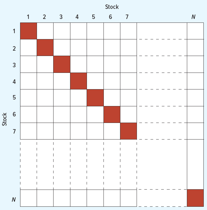
• Diagonal cells contain variance terms, and the off-diagonal cells contain the covariance terms
• As \(N\) assets increases, the number of terms outside the main diagonal increases more than the main diagonal.
• Therefore, the variance of a well-diversified portfolio is mostly determined by the covariances, and not the individual stock variance terms!

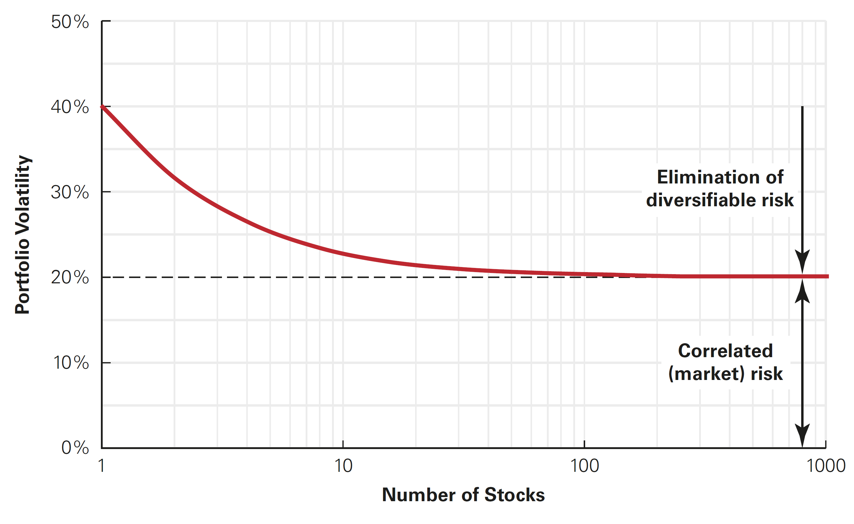
Limits to diversification

• How much of the variance of a portfolio we can eliminate through diversification?

• In practical terms:

  1. So, if you increase the size of your portfolio, the risk decreases (until to a certain amount)
  2. Usually, about half of the initial variance can be eliminated through diversification!

• Which type of risk is eliminated? Only the idiosyncratic risk! For example, firm-specific characteristics

• Which type of risk remains? Only the systematic risk! For example, economic conditions

\(\rightarrow\) For details regarding the mathematics behind risk minimization through diversification, see example for an equally-weighted portfolio in the Appendix

Limits to diversification, graphical interpretation

Choosing an Efficient Portfolio

Choosing Portfolios

• Now that we understand how to calculate the expected return and volatility of a portfolio, we can return to the main goal of the chapter: determine how an investor can create an efficient portfolio

• Let’s start of with the simplest case: create a portfolio with two stocks, Amazon and Ferrari. Previously, we’ve shown that, for the analysis period, we had the following results in terms of risk and return:

• Let’s create \(5\) different portfolios using \(\pm20\%\) of allocation weights in each asset

Choosing an Efficient Portfolio, continued

• We can plot this in a figure to show all possible risk \(\times\) return combinations

Choosing an Efficient Portfolio, 6 portfolios

Choosing an Efficient Portfolio, 11 portfolios

Choosing an Efficient Portfolio, >100 portfolios

Choosing an Efficient Portfolio

• As a financial manager, one crucial job you have is to find portfolios that are not sub-optimal
  1. For a given level of volatility, they deliver the highest possible return
  2. Alternatively, for a given level of return, they deliver the lowest possible volatility
• An easy what to look at this is to identify the minimum variance portfolio (MVP)
  1. This portfolio is, among all combinations, the one with the lowest volatility
  2. From there, if a given portfolio is riskier than the MVP, it needs to deliver higher returns!
  3. On the other hand, if a portfolio is riskier than the MVP and deliver the same/lower returns, it can be considered inefficient

\(\rightarrow\) In other words: investors should look only for efficient portfolios and will choose based on his specific preferences for risk!

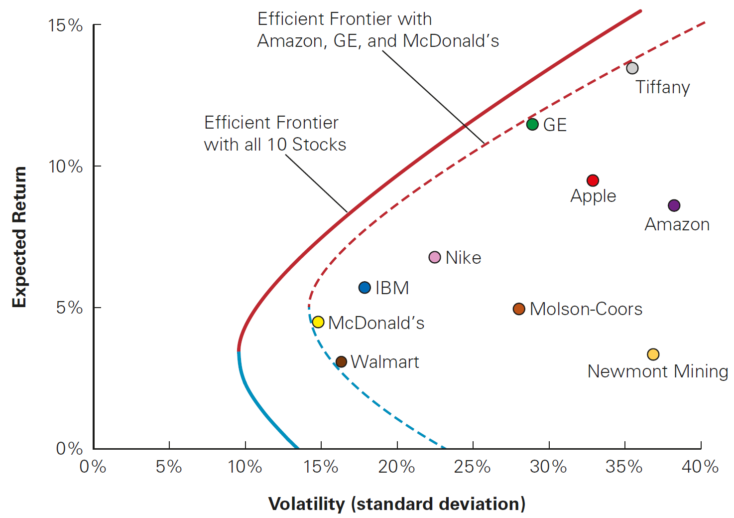
The Efficient Frontier

• In our example, we used only two assets. What happens when we increase the number of potential assets?

• Let’s replicate the same rationale by now investing our money in three possible stocks: Amazon,Ferrari, and VSCO

Which of these portfolios are efficient?

Which of these portfolios are efficient?

Choosing an Efficient Portfolio

• What happens when you continuously increase the number of assets?

  1. If you add stocks, you improve the frontier - i.e, you are able to create portfolios that span better options in terms of risk and return
  2. If you continue adding assets, you will have what is called Efficient Frontier

• The Efficient Frontier is the set of portfolios where:

  1. For a given level of volatility, you have the highest possible return among all portfolios with the same volalitity level
  2. For a given level of return, you have the lowest possible volatility among all portfolios with the same return level

• Based on this, is there a single portfolio in which all investors should hold? No! In practice, investors will choose among portfolios based on their specific preferences for risk and return

The Efficient Frontier

Risk-Free Saving and Borrowing

Risk-Free Saving and Borrowing

• Thus far, we have considered the risk and return possibilities that result from combining risky investments into portfolios

• By including all risky investments in the construction of the efficient frontier, we achieve the maximum diversification possible with risky assets

• In practice, however, we have the existence of risk-free assets, such as Treasury Bills, Treasury Bonds, Tesouro Direto etc

• Up to this point, we assumed that all the available assets had a minimum level of risk - for example, stocks

• In what follows, we will investigate what happens when we add the possibility of investing in a risk-free asset

• As you’ll see, when you add the risk-free asset, the implication is that there should only be only one efficient portfolio!

Risk-Free Saving and Borrowing

• Assume that you have a risk-free asset, such as a Treasury Bill, where the return is \(R_f\) and, by definition, has no risk
• You decided to invest a portion \(x\) of your holdings in the risky portfolio, and the remaining \(1-x\) in the risk-free asset
• The expected return from your new portfolio, which we’ll call \(R_{C}\), is:

\[E[R_{C}] = x \times E[R_p] + (1-x) \times R_f \]

• Rearranging terms, we have that:

\[ E[R_{C}] = x \times E[R_p] + R_f - x \times R_f\rightarrow R_f + x \times ( E[R_p] - R_f ) \]

Risk-Free Saving and Borrowing, continued

• Therefore, the expected return of a portfolio that contains risky assets and a risk-free asset is defined as:

\[ E[R_{C}] = R_f + x \times ( E[R_p] - R_f ) \]

• This equation shows that the expected return of your portfolio is the sum of:
  1. The risk-free rate; and
  2. A fraction of the portfolio’s risk premium, \(E[R_p] - R_f\), based on the fraction \(x\) that we invest in it
  3. A risk-premium is nothing more than the reward for bearing additional risk
• In other words, if you increase \(x\), your expected gains should increase because you’re more exposed to risk!

Risk-Free Saving and Borrowing, continued

• What happens to the volatility of a portfolio when you add the possibility of a risk-free asset?

• Remember that the risk free rate is assumed to have no risk, and therefore its variance is zero. As a consequence, the standard deviation of your portfolio that contains risky and risk-free assets is:

\[\small \sigma_{R_{C}} = \sqrt{(1-x)^2 \times \sigma^2_{R_f} + x^2 \times \sigma^2_{R_p} + 2 \times(1-x) \times x \times Cov(R_f, R_p)}\]

• Because \(\small \sigma^2_{R_f}=0\), this simplifies to:

\[\sigma_{R_{C}} = \sqrt{x^2 \times \sigma^2_{R_p}}\rightarrow x \times \sigma_{R_p}\]

• That is, the volatility is only a fraction of the volatility of the portfolio, based on the amount we invest in it

Risk-free combinations in practice

• In order to make this point clear, let’s go back to the efficient frontier built on top of the \(>100\) portfolios created using AMZN and RACE

• To facilitate the comparison, we’ll convert risk and return to annual terms

• If that is true, then the minimum-variance portfolio has:

  1. Annual Return \(\approx 3.82\%\)
  2. Annual Volatility \(\approx 3.24\%\)

• Suppose you have an risk-free investment opportunity, \(R_f\), that generates a risk-free return of 2%

• If that is true, we can think about all linear combinations of \([R_f,R_p]\) in which the returns are a weighted average of \(R_f\) and \(R_p\) and the volatility is only a fraction of \(R_p\)’s volatility

Risk-free combinations, graphical interpretation

Risk-Free Saving and Borrowing

• Remember that you can have short positions (“buying stocks on margin”) by:

  1. Borrowing at \(R_f\) to invest in a portfolio of risky assets
  2. Investing all your funds + the money you borrow in the portolio \(P\)

• If that is true, then you will have a negative weight in one asset (a short position) and a positive and >1 weight in the other asset

• If, as we’d imagine, \(R_p>R_f\) (i.e, the return of the minimum-variance portfolio is higher than \(R_f\), we could proceed by:

  1. Borrowing money at \(R_f\)
  2. Using this money to buy the minimum-variance portfolio, yielding a return of \(R_p\)

• In practice, because your return is a weighted average of \(R_f\) and \(R_p\) and \(R_p>R_f\), the linear combination line “extends” to the right as you are placing a higher weight on the asset with higher return

Buying stocks on margin

Selecting the portfolio

• As before, is there a single portfolio in which all investors should hold? No! In practice, investors will choose among portfolios based on their specific preferences for risk and return

• But you may have noticed something strange…the linear combination of \(R_f\) and \(R_p\) yields a sub-optimal portolio:

  1. There are many portfolios that yield higher returns than the minimum-variance portfolio (and are also riskier)
  2. However, if we want to have a lower risk, we can simply combine them with the risk-free asset, \(R_f\), and the volatility of the portfolio will be only a fraction of \(\sigma_P\)

• In other words, we could be better off if we had done a linear combination using a portfolio that yields a better risk \(\times\) return relationship!

• How can we find such a portfolio? We need to think about the point where \(\small \partial R_c/\partial\sigma_p\) is the highest - in graphical terms, the portfolio with the highest slope!

Buying stocks on margin

Sharpe-ratio and the tangent portfolio

• The ideal portfolio that we want to combine with the risk-free asset is called the tangent portfolio:
  1. It is tangent to the efficient frontier
  2. Because of that, it has the highest risk \(\times\) return combination
• To identify the tangent portfolio, we compute the Sharpe Ratio:

\[\text{Sharpe Ratio} = \frac{E[R_p]-R_f}{\sigma_{R_p}}\]

• In the Sharpe Ratio measures the ratio of reward-to-volatility provided by a portfolio:

1. It indicates the amount of excess returns a portfolio provides a “risk-adjusted” format
2. Higher Sharpe Ratio \(\rightarrow\) better risk \(\times\) return relationship

The use of the Sharpe Ratio

• What is the optimal portfolio to combine with the risk-free asset? The one with the highest Sharpe Ratio! This portfolio is the one where the line with the risk-free investment is tangent to the efficient frontier of risky investments. There are two important facts about it:

1. The tangent portfolio is efficient.

2. Once we include the risk-free investment, all efficient portfolios are combinations of the risk-free investment and the tangent portfolio.

• Therefore, all investors should have the tangent portfolio. All investors should combine the tangent portfolio with the risk free asset to adjust the level of risk.

• If you ignore the risk free asset, you have several efficient portfolios (efficient frontier). But once you combine with the risk free rate, there is only one!

The Efficient Portfolio and Required Returns

The Efficient Portfolio and Required Returns

• Suppose you hold a portfolio \(P\). How do you decide whether to include a new asset? In sum, you should include a new asset \(i\) in a portfolio if it increases the Sharpe Ratio of the resulting portfolio! Note that the new asset has the following properties:

  1. The excess return that this asset \(i\) brings is \(E[R_i] - R_f\)
  2. On the other hand, the risk that this asset \(i\) brings to your portfolio is \(\sigma_i \times corr(R_i,R_p)\) - see the Appendix for a detailed explanation

• Therefore, is the gain in excess return from investing in \(i\) sufficient to make up for the increase in risk? Think about this as your average grade in the university:

  1. If you take a test and obtains a score that is higher than your average grade \(\rightarrow\) your average grade will go up
  2. If, on the other hand, your score is lower than your average \(\rightarrow\) your average will go down
  3. Finally, if your score is exactly your average grade, your average grade remains unchanged

Efficient Portfolio and Required Returns, continued

• Going back to our portfolio: if you compute the Sharpe Ratio of \(i\) and \(P\), including \(i\) is beneficial if and only if:

\[\underbrace{\frac{E[R_i] - R_f}{\sigma_{R_i} \times corr(R_i,R_p)}}_{\text{Sharpe Ratio of } i} > \underbrace{\frac{E[R_p] - R_f}{\sigma_{R_p}}}_{\text{Sharpe Ratio of } P}\]

• Moving the denominator to the right-hand side, we have:

\[E[R_i] - R_f >\sigma_{R_i} \times corr(R_i,R_p) \times \frac{E[R_p] - R_f}{\sigma_{R_p}}\]

Efficient Portfolios and Required Returns, continued

\[E[R_i] - R_f > \underbrace{\frac{\sigma_{R_i} \times corr(R_i,R_p)}{\sigma_{R_p}}}_{\beta^P_i} \times (E[R_p] - R_f)\]

• Using a \(\beta\) notation and moving \(R_f\) to the right-hand-side:

\[ E[R_i] > R_f + \beta_i^P \times (E[R_p] - R_f) \]

Efficient Portfolio and Required Returns, continued

• To conclude, increasing the amount invested in \(i\) will increase the Sharpe Ratio of portfolio \(P\) if its expected return \(E[R_i]\) exceeds its required return given portfolio \(P\), defined as:

\[ E[R_i] > R_f + \beta_i^P \times (E[R_p] - R_f) \]

• The required return is the expected return that is necessary to compensate for the risk investment \(i\) will contribute to the portfolio.

1. It is is equal to the risk-free interest rate…
2. …plus the risk premium of the current portfolio, P…
3. … scaled by \(i\)’s sensitivity to \(P\), denoted by \(\beta_i^P\)

• If \(i\) expected return exceeds this required return, then adding more of it will improve the performance of the portfolio!

Efficient Port. and Required Returns, conclusion

• We saw what an efficient portfolio is and how to find it in terms of the Sharpe Ratio
• Based on this notion, this equation establishes the relation between an investment’s risk and its expected return:

\[R_i = R_f + \beta_i^P \times (E[R_p] - R_f)\]

• It states that we can determine the appropriate risk premium for an investment based on its \(\beta\) with the efficient portfolio

• In such a way, it enables us to “price” the required returns for investing in any asset based on the amount of required returns that are needed to improve the performance of an efficient portfolio

Practice

Important

Practice using the following links:

1. Multiple-choice Questions
2. Numeric Questions

Appendix

Proof - Variance of a sum of two random variables

Theorem I: the variance of the sum of two random variables equals the sum of the variances of those random variables, plus two times their covariance:

\[ \small \sigma^2(A+B) = \sigma^2_A + \sigma^2_B + 2\times Cov(A,B) \] Proof: variance is defined as:

\[ \small Var(X)=E[(X-E(X))]^2 \] Therefore, if \(X=A+B\), with \(A\) and \(B\) being two random variables:

\[ \small Var(X)=Var(A+B) = E[((A+B)-E(A+B))]^2 = E[(\underbrace{[A-E(A)]}_{\text{First Term}}+[\underbrace{B-E(B)}_{\text{Second Term}}])^2] \\ \] Which is now in the form \(\small (A+B)^2=A^2+B^2+2AB\). Using the fact that \(E(\cdot)\) is a linear operator, we can apply it to each of the terms:

\[ \small = \underbrace{E([A-E(A)]^2}_{\sigma^2_A}+\underbrace{E[B-E(B)]^2}_{\sigma^2_B}+2\times\underbrace{E[A-E(A)][B-E(B)]}_{Cov(A,B)} = \sigma^2_A + \sigma^2_B + 2\times Cov(A,B)\\ \]

Proof - Variance multiplied by a scalar

Theorem II: The variance scales upon multiplication with a constant:

\[ \sigma^2(\beta \times A ) = \beta^2\times \sigma^2_A \] Proof: define the variance in terms of \(\beta\) and \(A\):

\[ \sigma^2(\beta\times A)=E[\beta\times A-E(\beta\times A)]^2 \\ \] Since \(\beta\) is a constant, \(E[\beta]=\beta\) and we can write:

\[ E[\beta\times A - \beta\times E(A)]^2= E[\beta\times (A-E[A])]^2=\beta^2\times \underbrace{E(A-E[A])]^2}_{\sigma^2_A} \] Therefore, whenever there is a scale constant multiplying a random variable, it scales the variance: \(\beta^2 \times\sigma^2_A\)

Limits to diversification

• How much of the variance of a portfolio we can eliminate through diversification? To see that, assume that we hold a portfolio with equal weights \(\frac{1}{N}\) to all assets

1. In the diagonal, we have \(N\) boxes with \(\dfrac{1}{N^2}\times \overline{Var}\), where \(\overline{Var}\) is the average variance
2. Off the diagonal, we have \(N^2-N\) boxes with \(\dfrac{1}{N^2}\times \overline{Cov}\), where \(\overline{Cov}\) is the average covariance

• Therefere, you can rearrange terms to get:

\[ \small Var(R_p) = \bigg(N\times\dfrac{1}{N^2}\times \overline{Var}\bigg)+ \bigg[(N^2-N)\dfrac{1}{N^2}\times \overline{Cov}\bigg]\\ \small = \bigg(\frac{1}{N} \times \overline{Var}\bigg) + \bigg[\bigg(1-\frac{1}{N}\bigg) \times \overline{Cov}\bigg] \]

Limits to diversification, continued

• What happens if \(N\rightarrow\infty\)? If you look at our equation, you’ll see that only the covariance terms remain:

\[ \small \underset{N\rightarrow\infty}{\small Var(R_p)} = \bigg(\frac{1}{\infty} \times \overline{Var}\bigg) + \bigg[\bigg(1-\frac{1}{\infty}\bigg) \times \overline{Cov}\bigg]\rightarrow \overline{Cov} \]

Volatility of a large portfolio with arbitrary weights

• What if we don’t have an equally-weighted portfolio? As \(N\) increases, you can rewrite the variance of the portfolio¹ as:

\[\small \sigma^2_{R_p} = \sum_i w_i \times Cov(R_i,R_p)\]

• The variance of a portfolio approaches the weighted average covariance of each stock with the portfolio!

• Because \(\small Cov(R_i,R_P) = \sigma_i \times \sigma_p \times Corr_{i,p}\) you can also write it as:

\[\sigma^2_{R_p} = \sum_i x_i \times \sigma_{i} \times \sigma_{p} \times Corr_{i,p}\]

1. See Berk and DeMarzo (2023), pg. 409 for a detailed explanation.

Volatility of a large portfolio with arbitrary weights

• If we divide both sides of this equation by \(\sigma_{p}\), we find:

\[\sigma_{p} = \sum_i x_i \times \sigma_{i} \times Corr(R_i,R_p)\]

• Why this equation is important?

  1. It shows the amount of risk that each security brings to portfolio

  2. Each asset \(i\) contributes to the portfolio’s volatility according to its standard deviation (\(\sigma_i\)) scaled by its correlation with the portfolio

References

Berk, J., and P. DeMarzo. 2023. Corporate Finance, Global Edition. Global Edition / English Textbooks. Pearson. https://books.google.com.br/books?id=m78oEAAAQBAJ.

Brealey, R. A., S. C. Myers, and F. Allen. 2020. Principles of Corporate Finance. The Irwin/McGraw-Hill Series in Finance, Insurance, and Real Estate. McGraw-Hill Education. https://books.google.com.br/books?id=nsrHuwEACAAJ.